This Riddler is about microorganisms multiplying. Will they thrive or will the species go extinct?
At the beginning of time, there is a single microorganism. Each day, every member of this species either splits into two copies of itself or dies. If the probability of multiplication is p, what are the chances that this species goes extinct?
Here is my solution:
[Show Solution]
Here is a short and sweet solution to the problem. Let’s call $q$ the probability that the species eventually goes extinct. If a microorganism fails to multiply (probability $1-p$), then it goes extinct immediately. If it multiplies, we now have two microorganisms, each with probability $q$ of eventually going extinct. The probability that they both eventually go extinct is $q^2$ because they behave independently. Therefore, we can write the recursion:
\[
q = p\, q^2+(1-p)
\]This equation has two possible solutions: $q \in \{1, \tfrac{1}{p}-1\}$. Since probabilities cannot exceed $1$, the second solution only makes sense in the case where $p \ge \tfrac{1}{2}$. Therefore, the solution is:
\[
q = \begin{cases}
1 &\text{if }p < \tfrac{1}{2} \\
\tfrac{1}{p}-1 &\text{if }p \ge \tfrac{1}{2}
\end{cases}
\]Here is a plot showing what the probability of extinction looks like as a function of $p$, the probability of multiplication:
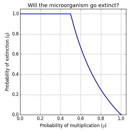
This is an interesting result because of the phase transition that occurs at $p=\tfrac{1}{2}$. If the probability of multiplication is less than one half, the species will always eventually go extinct. When the probability of multiplication is greater than one half, there is a nonzero chance that the population will grow enough that the species becomes “too big to fail”.
Here is a more technical (and more correct!) solution adapted from a comment by Bojan.
[Show Solution]
The previous approach obtains the correct answer, but the issue of which solution to the quadratic equation to pick still remains. This alternative approach obtains the correct answer using a generating function approach. Define the probability distribution:
\[
P_n(i) := (\text{probability there are }i\text{ microorganisms on day }n)
\]Now define the sequence of polynomials:
\[
Q_n(x) := \sum_{i=0}^\infty P_n(i)\, x^i
\]Then $Q_1(x) = x$, since there is one organism on day one. We can derive a recursive relation for the multiplication/exctinction process by thinking carefully about how the population can change from one day to the next. It’s not difficult to see that after the first timestep, the population must always be even. If the population is $2i$ at time $n+1$ and the population was $j$ at time $n$, then $j \ge i$. The probability that we transition from $j$ to $2i$ requires that exactly $i$ microorganisms multiply and the rest die. This can happen in ${j\choose i}$ ways, each with probability $p^i(1-p)^{j-i}$ (it’s a binomial distribution). Therefore, we have the recursion:
\[
P_{n+1}(2i) = \sum_{j=i}^\infty {j\choose i} p^i (1-p)^{j-i} P_n(j)
\]We can now use this fact to find a recursion for our generating function $Q_n.$ Again, we’ll make use of the fact that when $n>1$, there can only be an even number of microorganisms:
\begin{align}
Q_{n+1}(x)
&= \sum_{i=0}^\infty P_{n+1}(i)\, x^i\\
&= \sum_{i=0}^\infty P_{n+1}(2i)\, x^{2i}\\
&= \sum_{i=0}^\infty \sum_{j=i}^\infty {j\choose i} p^i (1-p)^{j-i} P_n(j)\, x^{2i} \\
&= \sum_{j=0}^\infty \sum_{i=0}^j {j\choose i} p^i (1-p)^{j-i} P_n(j)\, x^{2i} \\
&= \sum_{j=0}^\infty P_n(j) \sum_{i=0}^j {j\choose i} (px^2)^i (1-p)^{j-i} \\
&= \sum_{j=0}^\infty P_n(j) \left(px^2+(1-p)\right)^j \\
&= Q_n(px^2+(1-p))
\end{align}A couple notes: in the fourth step, we interchanged the order of summation for $i$ and $j$ and in the sixth step we used the binomial theorem. Summarizing, we conclude that
\[
Q_{n+1}(x) = Q_n(px^2+(1-p))
\]The probability of extinction after $n$ timesteps is $P_n(0)$ (the probability that the population is zero). We’re interested in the limit of $P_n(0)$ as $n$ goes to infinity. This is equivalent to the constant term in our sequence of polynomials, so we are interested in finding: $\lim_{n\to\infty} Q_n(0)$. Let’s take a look at the first few terms:
\begin{align}
Q_1(x) &= x\\
Q_2(x) &= px^2 + (1-p)\\
Q_3(x) &= p\left(px^2 + (1-p)\right)^2 + (1-p)\\
Q_4(x) &= p\left(p\left(\left(px^2 + (1-p)\right)^2 + (1-p)\right)^2 + (1-p)\right)^2 + (1-p)\\
\dots
\end{align}Evaluating at zero, we get:
\begin{align}
Q_1(0) &= 0\\
Q_2(0) &= 1-p\\
Q_3(0) &= p(1-p)^2 + (1-p)\\
Q_4(0) &= p\left( p(1-p)^2 + (1-p)\right)^2 + (1-p)\\
\dots
\end{align}The pattern is clear (we could also prove it using induction). If we define $q_n := Q_n(0)$, the recursion satisfied is:
\[
q_{n+1} = p\, q_n^2 + (1-p)\qquad\text{with: }q_1 = 0
\]Any limit $q_n \to q$ of this recursive sequence must satisfy the fixed point equation $q = p\,q^2+(1-p)$. This is precisely what we found in our first solution to the problem! So what’s the big deal? Why did we go through all this trouble to arrive at the same answer?? This recursion actually tells us something more that just the limiting case. It tells us how we approach the limiting case. In other words, it gives us the dynamics.
Let’s take a closer look at these dynamics in the neighborhood of the two fixed points $q=1$ and $q=\tfrac{1}{p}-1$. If we let $\delta_n := q_n-1$, we can rewrite the recursion as:
\[
\delta_{n+1} = 2p\, \delta_n + p\, \delta_n^2
\]Of course, if $\delta_n=0$ (i.e. $q_n=1$), then it will remain at $1$ forever. But what if we are merely close to this fixed point? Then $\delta_n \approx 0$ and we have $\delta_{n+1} \approx 2p\,\delta_n$. Notice that when $p > \tfrac{1}{2}$ If $\delta_n$ is close to zero, it will never get closer because $2p > 1$. These dynamics are unstable.
Now take a look at the other fixed point. If we let $\epsilon_n := q_n-\tfrac{1}{p}+1$, then we can rewrite the recursion as:
\[
\epsilon_{n+1} = 2(1-p)\epsilon_n + p\,\epsilon_n^2
\]If we are close to this fixed point, then $\epsilon_n \approx 0$ and we have $\epsilon_{n+1} \approx 2(1-p)\epsilon_n$. This time, when $p > \tfrac{1}{2}$, we have $2(1-p) < 1$. In other words, if we are close, we continue to get closer! These dynamics are stable.
This stability argument explains why we converge to $\tfrac{1}{p}-1$ rather than $1$ in the case where $p>\tfrac{1}{2}$. If we consider the other case, where $p<\tfrac{1}{2}$, the stability flips. The first fixed point becomes stable and the second one becomes unstable. This transition in stability of the dynamics explains the abrupt transition in the plot at the point $p=\tfrac{1}{2}$.