You and four statistician colleagues find a \$100 bill on the floor of your department’s faculty lounge. None of you have change, so you agree to play a game of chance to divide the money probabilistically. The five of you sit around a table. The game is played in turns. Each turn, one of three things can happen, each with an equal probability: The bill can move one position to the left, one position to the right, or the game ends and the person with the bill in front of him or her wins the game. You have tenure and seniority, so the bill starts in front of you. What are the chances you win the money? What if there were N statisticians in the department?
Here is my solution to the first part, assuming five statisticians.
[Show Solution]
We can use an approach similar to the one used in the solution to the Monsters’ Gems problem. Namely, let’s arrange the statisticians around the table, starting at $0$ for the one with tenure, and moving clockwise labeling the others $1$, $2$, $3$, and $4$. We’ll let $x_i$ denote the probability that the tenured statistician will win given that the \$100 bill is currently laying in front of statistician $i$. We’d like to find $x_0$. Based on the rules of the game, we can write recursions that define each $x_i$ in terms of the others. First, we have:
\[
x_0 = \frac{1}{3} + \frac{1}{3} x_1 + \frac{1}{3} x_4
\]because there are three outcomes: the tenured statistician (number $0$) wins the \$100 bill, or it gets passed clockwise to statistician $1$, or it gets passed counterclockwise to statistician $4$. Each of these happens with an equal probability of $\tfrac{1}{3}$. When the bill is in front of statistician $1$, we have:
\[
x_1 = \frac{1}{3} x_0 + \frac{1}{3} x_2
\]the logic is similar here, except one of the three outcomes is now that the tenured statistician wins nothing. The other two outcomes involve passing the bill either clockwise to statistician $2$ or counterclockwise back to statistician $0$. We can write similar equations for the other three statisticians, and rearranging the equations, we obtain:
\begin{align}
3x_0-x_1-x_4 &= 1 \\
3x_1-x_2-x_0 &= 0 \\
3x_2-x_3-x_1 &= 0 \\
3x_3-x_4-x_2 &= 0 \\
3x_4-x_0-x_3 &= 0
\end{align}These are five equations in as many unknowns, which we can solve by substitution or by a variety of other methods. The final result is:
\[
x_0 = \tfrac{5}{11} \approx 0.4545,
\quad
x_1=x_4=\tfrac{2}{11} \approx 0.1818,
\quad
x_2=x_3=\tfrac{1}{11} \approx 0.0909
\]Therefore, we conclude that:
$\displaystyle
\text{there is a 45.45% chance the tenured statistician will win}
$
A useful observation: because of the circular symmetry in the problem, the following two probabilities are equal:
- the probability that statistician $i$ wins given that the bill starts in front of statistician $0$.
- the probability that statistician $0$ wins given that the bill starts in front of statistician $i$.
So we can think of $x_i$ in either of these two equivalent ways. Consequently, each immediate neighbor of statistician $0$ has an 18.18% chance of winning the \$100 bill, and the two remaining statisticians each have a 9.09% chance of winning.
Here is my solution to the second part, assuming $N$ statisticians.
[Show Solution]
If there are $N$ statisticians, we can follow an approach similar to the $5$-statistician case. The result is $N$ equations:
\begin{align}
3x_0-x_1-x_{N-1} &= 1 \\
3x_1-x_2-x_0 &= 0 \\
3x_2-x_3-x_1 &= 0 \\
\vdots & \\
3x_{N-1}-x_0-x_{N-2} &= 0
\end{align}This is analogous to the $5$-statistician case except now we have $N$ equations in $N$ unknowns. Although we could solve them for each $N$ separately, this won’t help us find a closed-form solution. Instead, realize that this is simply a linear recurrence relation, albeit a nonstandard one. Rewrite it as follows:
\[
3x_k-x_{k-1}-x_{k+1} = \delta_k\qquad\text{for: }k=0,1,\dots
\]Here, $\delta_k$ is the Kronecker Delta ($1$ when $k=0$ and 0 otherwise). So technically, this is a linear non-homogeneous recurrence relation with constant coefficients. The twist is that such recurrences typically have initial conditions, e.g. we might know $x_0$ and $x_1$ and seek to find the rest of the terms. In this case, we have a boundary condition instead. Namely, we know that $x_0 = x_N$. This is no problem; we may still use the standard approach for solving recurrence relations. These are also known as eventually periodic sequences.
The standard approach is to consider the homogeneous version first, and and assume a solution of the form $\lambda^k$. This results in the characteristic polynomial $\lambda^2-3\lambda+1 = 0$. The roots of this polynomial are $a = \frac{3-\sqrt{5}}{2}$ and $a^{-1} = \frac{3+\sqrt{5}}{2}$. It turns out we can use the standard form
\[
x_k = p a^k + q a^{-k}
\]in spite of the non-homogeneity. In order to solve for $p$ and $q$, we impose the two constraints:
\begin{align}
3x_0-x_1-x_{N-1}&=1 && \text{(special behavior at }k=0\text{)}\\
x_0-x_{N} &= 0 && \text{(periodicity requirement)}
\end{align}Substituting our proposed form for $x_k$, we obtain the equations:
\begin{align}
3(p+q)-\left(pa+qa^{-1}\right)-\left(pa^{N-1}+qa^{-N+1}\right) &= 1 \\
(p+q)-\left(pa^N+qa^{-N}\right) &= 0
\end{align}These are linear equations in $p$ and $q$, which we can solve and substitute the result back into the expression for $x_k$, yielding:
\[
x_k = \frac{a^{N-k}+a^k}{(3-2a)+a^N(3-2a^{-1})}
\]Substituting $a = \frac{3-\sqrt{5}}{2}$ and simplifying, we obtain the general solution for the recurrence relation in closed form:
$\displaystyle
\begin{aligned}
&\text{the }k^\text{th}\text{ statistician wins with probability }\\
&\quad x_k = \frac{1}{\sqrt{5}}\left(\frac{3-\sqrt{5}}{2}\right)^k\left(
\frac{1 + \left(\frac{3-\sqrt{5}}{2}\right)^{N-2k}}{1-\left(\frac{3-\sqrt{5}}{2}\right)^N}\right)
\end{aligned}
$
We can verify that the formula satisfies $x_k = x_{N-k}$, which makes sense because of the circular symmetry in the problem, and that $\sum_{k=0}^{N-1}x_k = 1$ because the probabilities must sum to $1$. We can also see that as $N\to\infty$ the final bracketed term vanishes and we are left with a much simpler exponential function of $k$.
For the brave and curious, this next section explores connections between the problem and Fourier Transforms, complex analysis, and Chebyshev polynomials. Fair warning: advanced math!
[Show Solution]
In what follows, I’ll present several alternative approaches to solving the problem: a DFT approach, a complex analysis approach for finding the limiting distribution, and connections to Chebyshev polynomials.
Using the same approach as in the first and second solutions, we can write equations relating $x_0,x_1,\dots,x_{N-1}$ for the $N$ statisticians. In matrix form, these are:
\[
\begin{bmatrix}
3 & -1 & 0 & \dots & -1 \\
-1 & 3 & -1 & & 0 \\
0 & -1 & \ddots & \ddots & \vdots \\
\vdots & & \ddots & 3 & -1 \\
-1 & 0 & \dots & -1 & 3
\end{bmatrix}
\begin{bmatrix} x_0\\x_1\\x_2\\\vdots\\x_{N-1} \end{bmatrix} =
\begin{bmatrix} 1\\0\\0\\\vdots\\0 \end{bmatrix}
\]We’ll just write $Ax=b$ for short. The matrix $A$ has what is known as a circulant structure: it’s constant along its major diagonals and it “wraps around”. That is, if you index the entries as $(i,j)$ with $0\le i,j \le N-1$, then you would have $A(i,j) = A(i+1,j+1)$, where the indices are written modulo $N$. Another way of saying this is that the circulant matrix is characterized by its first column; each other column is a wrap-around shifted version of the previous column.
An obvious way to solve this system of equations is to simply invert the matrix, but this requires solving a different problem for each $N$ and these problems will get progressively more difficult as $N$ gets larger. It turns out there is an efficient way of exploiting the circulant structure.
Discrete Fourier Transforms
The first solution I’ll present uses Discrete Fourier Transforms. This won’t lead to a closed-form solution, but it’s nonetheless interesting! We’ll start with an amazing fact about circulant matrices: every circulant matrix has the same eigenvectors. Specifically, for any circulant $A$, we have:
\[
A = F^* \Lambda F
\]where $F_{k\ell} = \tfrac{1}{\sqrt{N}} \omega^{k\ell}$, where $\omega = \exp\left(\frac{2\pi i}{N}\right)$. The matrix $F$, which diagonalizes $A$, is known as the Discrete Fourier Transform (DFT) matrix. Notice that $F$ does not depend on $A$ at all!
If we let $c = \begin{bmatrix}c_0 & c_1 & \dots & c_{N-1}\end{bmatrix}^\mathsf{T}$ be the first column of $A$, the eigenvalues of $A$ are in the diagonal matrix $\Lambda$, and given by:
\[
\Lambda_{kk} = c_0 + c_{N-1} \omega + c_{N-2} \omega^2 + \dots c_2 + \omega^{N-2} + c_1 \omega^{N-1}
\]
By applying the diagonalization, $Ax=b$ becomes $F^* \Lambda F x = b$, which we can rearrange to obtain $x = F^* \Lambda^{-1} F b$. Here, we took advantage of the fact that $F$ is orthogonal, so $F^{-1} = F^*$. By substituting the definitions of $F$ and $\Lambda$ and expanding, we obtain:
\[
x_k = \frac{1}{N} \sum_{\ell = 0}^{N-1} \omega^{-k\ell}\left( 3-\omega^\ell-\omega^{-\ell}\right)^{-1},
\qquad\text{where }\omega = \exp\left(\tfrac{2\pi i}{N}\right)
\]Staring at this carefully, we notice that the imaginary parts cancel by odd symmetry, and we can express the result in terms of trig functions:
\[
x_k = \frac{1}{N} \sum_{\ell=0}^{N-1} \frac{\cos\left(\tfrac{2\pi k \ell}{N}\right)}{3-2\cos\left(\tfrac{2\pi\ell}{N}\right)}
\qquad\text{for }k=0,1,\dots,N-1
\]Later, we will see how to find a closed-form expression for this sum. As a sanity check, we can substitute $N=5$ and verify that we obtain the same $x_k$ as in the first part of the problem, so we’re in good shape! Computing the sum for particular values of $N$ and $k$ can be done efficiently if we exploit the circulant nature of the problem. We’re getting a little far afield here so I’ll refer the interested reader to this article that summarizes solving linear equations when the $A$ matrix is circulant. The result is that if $\mathcal{F}$ is the Discrete Fourier Transform operator, then we have:
\begin{align}
Ax=b &\iff x = \mathcal{F}^{-1} \left( \frac{ \mathcal{F}(b) }{ \mathcal{F}(c) } \right) \\
\end{align}where the division is performed element-wise. Here is Matlab code that uses the above approach to solve the problem numerically for any $N$:
N = 5;                        % number of statisticians
b = zeros(N,1); b(1) = 1;     % the "b" matrix in Ax=b
c = [3;-1;zeros(N-3,1);-1];   % the first column of the "A" matrix in Ax=b
x = ifft( fft(b)./fft(c) )    % that's it!
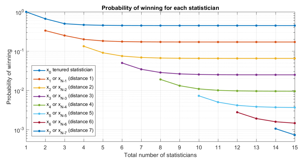
Matlab uses the FFT (Fast Fourier Transform) algorithm, which is a very efficient way of computing the Discrete Fourier Transform or its inverse. Here is a plot illustrating the expected winnings of the first few statisticians as a function of the total number of statisticians.

As we can see, the expected winnings for each statistician shrinks as we add more statisticians, but the values quickly settle to their limiting values as $N$ gets large. The limiting values appear to be evenly spaced on this logarithmic plot… Let’s look at that more closely!
Infinite Limit
We might ask what the probability of winning for each statistician looks like as $N$ gets very large. To handle this case, we can use the fact that our expression for $x_k$ as a sum becomes an integral as $N\to\infty$.
\[
\bar x_k = \lim_{N\to\infty} \frac{1}{N} \sum_{\ell=0}^{N-1} \frac{\cos\left(\tfrac{2\pi k \ell}{N}\right)}{3-2\cos\left(\tfrac{2\pi\ell}{N}\right)}
= \int_0^1 \frac{\cos(2\pi k u)}{3-2\cos(2\pi u)}\,du
\]Although it’s possible to evaluate this integral via traditional means by using Chebyshev polynomials, the most direct way is via complex analysis. To do this, we’ll return to the complex form of the integral by making the substitution $z = e^{2\pi i u}$ and $dz = 2\pi i z\, du$. As $u$ ranges from $0$ to $1$, $z$ travels counterclockwise along the circle $|z|=1$ in the complex plane. After simplification, we obtain the following contour integral:
\[
\bar x_k = \frac{1}{2\pi i}\oint_{|z|=1} \frac{-z^{k}}{z^2-3z+1}\,dz
\]This integral may be evaluated using Cauchy’s Residue Theorem. Notice that the denominator factors as $z^2-3z+1 = (z-a)(z-a^{-1})$ where $a = \frac{3-\sqrt{5}}{2}$ and $a^{-1} = \frac{3+\sqrt{5}}{2}$. Since $z=a$ is the only pole of the integrand inside the unit disc, it follows from the residue theorem that
\[
\bar x_k = \lim_{z\to a} \frac{-z^k}{z^2-3z+1}(z-a) = \frac{-a^k}{a-a^{-1}} = \frac{a^k}{\sqrt{5}}
\]We therefore conclude that
$\displaystyle
\begin{aligned}
&\text{in the limit }N\to\infty\text{, the }k^\text{th}\text{ statistician wins with probability}\\
&\quad\bar x_k = \frac{1}{\sqrt{5}}\left(\frac{3-\sqrt{5}}{2}\right)^k
\end{aligned}
$
Note that this matches the limit found in our second solution. In particular, the tenured statistician ($k=0$) will win the \$100 bill with probability $\frac{1}{\sqrt{5}} \approx 44.72\%$ if there are infinitely many statisticians participating in the game. The exponential form for $\bar x_k$ also explains why the plot we showed earlier has evenly spaced lines when we use a log-scale for the y-axis!
Chebyshev Connection
We’ll look at another way of solving the limiting integral
\[
\bar x_k = \int_0^1 \frac{\cos(2\pi k u)}{3-2\cos(2\pi u)}\,du
\]Make the substitution $v = 2\pi u$ and use the fact that the integrand is symmetric so we can split the range in half and get the same result:
\[
\bar x_k = \frac{1}{\pi}\int_0^\pi \frac{\cos(k v)}{3-2\cos(v)}\,dv
\]It turns out that $\cos(k v)$ can be expressed as $T_k(\cos(v))$, where $T_k$ is a polynomial. For example, $\cos(2v) = 2\cos^2(v)-1$ and so $T_2(x) = 2x^2-1$. The polynomials $T_k$ are called Chebyshev polynomials. By making the substitution $y = \cos(v)$, our integral becomes:
\[
\bar x_k = \frac{1}{2\pi}\int_{-1}^1 \frac{T_k(y)}{(\tfrac{3}{2}-y)\sqrt{1-y^2}}\,dy
\]Doesn’t seem like we’ve made any progress, except that we’ve eliminated all of the trig functions. We can evaluate the integral for each $k$ on an individual basis, but it turns out there is a closed-form expression for the above integral, which stems from the fact that it is a Hilbert Transform. The formula is given in the following manuscript (see equation (7.4)).
We end up with the formula
\[
\bar x_k = -\frac{1}{2} U_{k-1}(\tfrac{3}{2}) + \frac{1}{\sqrt{5}} T_k(\tfrac{3}{2})
\]where $U$ is the Chebyshev polynomial of the second kind. This is simpler than the integral, but we’re not done yet! Chebyshev polynomials have closed-form expressions. Namely, when $|x|\ge 1$, we have:
\begin{align*}
T_k(x) &= \frac{\left(x+\sqrt{x^2-1}\right)^k + \left(x-\sqrt{x^2-1}\right)^k}{2} \\
U_{k-1}(x) &= \frac{\left(x+\sqrt{x^2-1}\right)^k – \left(x-\sqrt{x^2-1}\right)^k}{2\sqrt{x^2-1}}
\end{align*}Substituting these expressions into the above formula for $\bar x_k$, we obtain:
\[
\bar x_k = \frac{1}{\sqrt{5}}\left(\frac{3-\sqrt{5}}{2}\right)^k
\]which is the same as what we found using the complex analysis approach. Whew!
I suppose for challenging problems like this one, people tend to grab the tools they are most comfortable with. My aim was to stick with Linear Algebra tools. (Shame on me for recognizing that the fundamental matrix for the markov chain was symmetric, but missing the circulant structure.)
There is some very good stuff in this post… but no mention of Fibonacci numbers?? For better or worse, this led me to post my solution in full, below.
My approach may seem a touch opaque, but it is a considerably simpler solution — no integrals or required use of the infinite.
Here it is:
Consider a function, f, that takes in some scalar, c, and a vector, x, and returns a scalar. Note that c = n // 2 (i.e. integer division of n, so for example, if n= 5, c = 2).
here $f(c, x) = \left[\begin{matrix}1\\0\end{matrix}\right]^T * Y^{c} x $
where $x = \left[\begin{matrix}x0\\x1\end{matrix}\right]$ and
$Y = \left[\begin{matrix}3 & -1\\1 & 0\end{matrix}\right]$
Note: we may also rewrite our function purely in terms of scalars as f(c, x0, x1)
Eventually we will diagonalize Y, such that $Y^c = PD^{c}P^{-1}$
Also note: Y looks kind of a like a demented fibonacci matrix, and indeed if you look at the output of:
for c in range(1, somevalue):
# not coincidentally, these are used in the final answer
print f(c, x0= 1, x1 = 1)
print f(c, x0= 0, x1 =-1)
(edit: I could not get the indentation for the above code block to show up quite right.)
you will actually recover the fibonacci numbers sequence.
(Note: technically what follows applies to cases of having n being odd — a small tweak can adjust it for the case of n being even.)
Now to go from all this to the final probability:
First: The ‘raw frequency’ for the 0’th statistician to win is given by $f(c= n//2, x0=1, x1 =1)$ i.e. the first print stmt in the above for loop.
The sum of the ‘raw frequencies’ for all the other statisticians to win is: $2*(c=n//2, x0= 0, x1 = -1)$ (i.e. the second print stmt in the above for loop, times 2). Note that we can use linearity and apply the 2 inside the function, but I left it outside as it makes things / underlying patterns easier to follow. It’s also worth remembering that when n is odd, setting aside the 0’th statistician, everyone has a ‘twin’ who has the exact same expectations, and that is what the scalar of 2 is for.
So the probability that the zero’th statistician wins is $\frac{numerator}{denominator}$
where $numerator = f(c= n//2, x0=1, x1 =1)$
and $denominator = f(c= n//2, x0=1, x1 =1) + 2(c=n//2, x0= 0, x1 = -1)$
Now. If you go through the effort of diagonalizing Y, and working through all of the algebra, you will get a closed form expression of
prob player zero wins = $p(win) = \frac{- 3571 \left(- \sqrt{5} + 3\right)^{c} + 1597 \sqrt{5} \left(- \sqrt{5} + 3\right)^{c} – 1364 \left(\sqrt{5} + 3\right)^{c} + 610 \sqrt{5} \left(\sqrt{5} + 3\right)^{c}}{- 7985 \left(- \sqrt{5} + 3\right)^{c} + 3571 \sqrt{5} \left(- \sqrt{5} + 3\right)^{c} – 1364 \sqrt{5} \left(\sqrt{5} + 3\right)^{c} + 3050 \left(\sqrt{5} + 3\right)^{c}}
$
The above probably can be further simplified using closed form expressions for fibonnaci numbers, but further simplifying fractions is something for another day.
Now that we have a nice finite closed form expression, we may take a limit and get
$\lim_{c \to \infty}p(win) = – \frac{-682 + 305 \sqrt{5}}{-1525 + 682 \sqrt{5}}$
which I realized is equivalent to the much simpler $\frac{1}{\sqrt{5}}$ only after reading your post. It is remarkable how useful this limit is — it is an extremely close approximation even for say N = 9 or N = 10.
Thanks! Several others mentioned connections to the Fibonacci numbers. For example here and here. I thought my post was already too long so I just stopped 🙂
Yea… it looks like Rajeev nailed it. I suppose I’d express the solution for the odd numbers as:
$\frac{F_n }{3 F_n – 2 F_{n-2}}$
but this really is a distinction without a difference
Right, if we notice that the Fibonacci sequence satisfies
\begin{equation}
F_{n+4}=F_{n+3}+F_{n+2}=2F_{n+2}+F_{n+1}=3F_{n+2}-F_n
\end{equation}
we see that the recursion $a_{n+2}=3a_{n+1}-a_n$ is fulfilled both by the odd-numbered $(1,2,5,13,…)$ and the even-numbered $(1,3,8,21,…)$ Fibonacci numbers, and consequently by any linear combination of these.
Rajeev’s result follows then quite easily.
and for what it’s worth, $\frac{3\mp\sqrt{5}}{2} = \left(\frac{1\pm\sqrt{5}}{2}\right)^2$, the square of the golden ratio and its negative inverse, which have the obvious connection to the Fibonacci sequence.
Beautiful analysis as always!
Here is yet another method of solution, which in some ways is a little simpler. Let’s generalize to the case that we pass left with probability x, right with probability y, and stop with probability 1-x-y. The probability of a total of L left passes and R right passes before stopping is
p[L,R] = (1-x-y) x^L y^R n[L,R],
where n[L,R] is the number of inequivalent arrangements of the passes; this number is (L+R)!/(L!R!), but we will not need this formula. Instead, all we will need to know is that the probabilities p[L,R] must sum to one, so it must be that
Sum_(L,R) x^L y^R n[L,R] = 1/(1-x-y),
where each sum runs from zero to infinity. To get x_k, the probability that the k^th statistician wins, we must sum only those probabilities for which L-R-k is a multiple of N. We can do this by inserting in the sum a factor of
(1/N)Sum_(j=0 to N-1) w^(j*(L-R-k)),
where w = exp(2 pi i/N). This sum equals one if L-R-k is a multiple of N, and vanishes otherwise (by usual properties of the roots of unity). Now we have
x_k = (1-x-y)(1/N)Sum_(j=0 to N-1) Sum_(L,R) w^(-kj) (x w^j)^L (y w^-j)^R n[L,R].
We already know how to do the sums over L and R, so we have
x_k = (1-x-y)(1/N)Sum_(j=0 to N-1) w^(-kj)/(1 – x w^j – y w^-j).
For the case x=y=1/3, this is the same as your result from the discrete Fourier transform.
neat! Thanks for sharing!
I like the closed form solution, but the first step — getting kth player winning probability for infinite n — can be simplified (though more complex solutions can also be informative).
Let E(k) be the expected number times player k will get the bill. We have,
E(0) = 1+E(1)*2/3 (since player 0 gets the bill initially and E(1)=E(-1))
E(k) = 1/3*(E(k-1)+E(k+1)) (k>0)
This is a linear homogeneous recurrence relation. The standard way of solving it is first finding solutions with E(k)/E(k-1) constant, say E(k)/E(k-1)=r. We have $r = 1/3+(1+r^2)$, with the solutions $r_1 = 3/2-\sqrt{5}/2$ and $r_2=3/2+\sqrt{5}/2$. Thus, $E(k) = c_1 k^{r_1}+c_2 k^{r_2}$. $c_2 = 0$ since $r_2>1$ and the sum of all E(k) is finite.
$c_1 = E(0) = 1+E(1) 2/3 = 1+c_1 r_1 2/3$, so $c_1 = 3/\sqrt{5}$.
Each time the player gets the bill, he keeps it with probability 1/3, so the probability that player k (the first player is 0) gets the bill is $E(k)/3 = 1/\sqrt{5} (3/2-\sqrt{5}/2)^k$.
[the above comment with some markup fixed]
I like the closed form solution, but the first step — getting kth player winning probability for infinite n — can be simplified (though more complex solutions can also be informative).
Let E(k) be the expected number times player k will get the bill. We have,
E(0) = 1+2/3*E(1) (since player 0 gets the bill initially and E(1)=E(-1))
E(k) = 1/3*(E(k-1)+E(k+1)) (k>0)
This is a linear homogeneous recurrence relation. The standard way of solving it is first finding solutions with E(k)/E(k-1) constant, say E(k)/E(k-1)=r. We have $r = frac{1}{3}(1+r^2)$, with the solutions $r_1 = 3/2-\sqrt{5}/2$ and $r_2=3/2+\sqrt{5}/2$. Thus, $E(k) = c_1 r_1^k+c_2 r_2^k$. Here, $c_2 = 0$ since $r_2>1$ and the sum of all E(k) is finite.
$c_1 = E(0) = 1+\frac{2}{3} E(1) = 1 + \frac{2}{3} c_1 r_1$, so $c_1 = 3/\sqrt{5}$.
Each time the player gets the bill, he keeps it with probability 1/3, so the probability that player k (the first player is 0) gets the bill is $E(k)/3 = \frac{1}{\sqrt{5}} (3/2-\sqrt{5}/2)^k$.
Correction: $r = \frac{1}{3}(1+r^2)$
Here is a different solution if we just want the first player win probability given n statisticians.
First use symmetry to merge pairs of players that are at the same distance from you:
you: probability 1/3 – keep the bill, 2/3 – move the bill
each middle player: 1/3 keep, 1/3 move left, 1/3 move right
rightmost player (odd n): 1/2 keep, 1/2 move (1/2 = 1/3+1/9+1/27+…).
rightmost player (even n): 1/3 keep, 2/3 move
Next, recursively merge the rightmost player with the player next to him. Let p be the probability that the rightmost player keeps the bill (and 1-p probability to move the bill to the neighbor).
1/3 move right → 1/3*p keep, 1/3*(1-p) stay until the next round
combined: 1/3 move left, 1/3+1/3*p keep, 1/3*(1-p) stay
Eliminate stay by normalizing the other options to 1: (1/3+1/3*p)/(1/3+1/3+1/3*p) = (p+1)/(p+2) keep
Final step (two players; if the second player has the bill, he keeps it with probability p and otherwise passes it to the first player):
1/3 – keep, 2/3*p – drop (the second player keeps the bill), 2/3*(1-p) – stay
Keep probability = 1/3/(1/3+2/3*p) = 1/(1+2*p)
Computation of the probability that the first player keeps the bill (‘=’ is used as assignment):
n is odd: p = 1/2
n is even: p = 1/3
repeat floor(n/2)-1 times: p = (p+1)/(p+2)
return 1/(1+2p)
Notes:
* For n=5, the result is 5/11.
* As n approaches infinity, p approaches (sqrt(5)-1)/2 (by solving the equation p=(p+1)/(p+2)), and the probability that the first player keeps the bill approaches 1/sqrt(5).
* To get the winning probability of the kth player, we can repeatedly merge the first player with the second one, though we have to keep track of two probabilities (basically, transmission and reflection probability).
* Given arbitrary time-independent probabilities for choosing the next player, the probability that the first player gets the bill can be found by considering $p_i$ — probability that player 1 gets the bill if the current player is i, and setting up a linear system in n variables (corresponding to one step) that relates the $p_i$.
Fibonacci and Lucas Numbers:
If p is a/b, the next p is (p+1)/(p+2) = (a+b)/(a+2b), so numerator1,denominator1,numerator2,denominator2,… form a Fibonacci recurrence.
For odd n, this corresponds to the Fibonacci sequence ($F_1=1$,$F_2=1$,$F_n=F_{n-1}+F_{n-2}$): $p = F_{n-1}/F_n$, and the answer is $F_n/(F_n+2 F_{n-1}) = F_n/(F_{n+1}+F_{n-1}) = F_n/L_n$.
For even n, this corresponds to the Lucas sequence ($L_1=1$,$L_2=3$,$L_n=L_{n-1}+L_{n-2}$): $p = L_{n-1}/L_n$, and the answer is $L_n/(L_n+2 L_{n-1}) = L_n/(L_{n+1}+L_{n-1}) = \frac{1}{5} L_n/F_n$.