When you roll a die “with advantage,” you roll the die twice and keep the higher result. Rolling “with disadvantage” is similar, except you keep the lower result instead. The rules further specify that when a player rolls with both advantage and disadvantage, they cancel out, and the player rolls a single die. Yawn!
There are two other, more mathematically interesting ways that advantage and disadvantage could be combined. First, you could have “advantage of disadvantage,” meaning you roll twice with disadvantage and then keep the higher result. Or, you could have “disadvantage of advantage,” meaning you roll twice with advantage and then keep the lower result. With a fair 20-sided die, which situation produces the highest expected roll: advantage of disadvantage, disadvantage of advantage or rolling a single die?
Extra Credit: Instead of maximizing your expected roll, suppose you need to roll N or better with your 20-sided die. For each value of N, is it better to use advantage of disadvantage, disadvantage of advantage or rolling a single die?
Here is a detailed derivation of the relevant probabilities:
[Show Solution]
We’ll use the following notation:
\begin{align}
f_k &= \mathbf{Prob}(X=k) & &\text{(probability mass function, pmf)} \\
F_k &= \mathbf{Prob}(X\leq k) & &\text{(cumulative mass function, cmf)} \\
\bar F_k &= \mathbf{Prob}(X\geq k) & &\text{(complementary cmf)}
\end{align}where $X$ is the outcome of a single roll of a fair $n$-sided die. Since it’s a fair die, these are:
\[
f_k=\frac{1}{n}, \qquad F_k=\frac{k}{n}, \qquad \bar F_k=\frac{n-k+1}{n}.
\]Let’s tackle the more complicated cases one by one. For the other events of interest, we’ll use similar notation but with superscripts “A” (advantage), “D” (disadvantage), “AD” (advantage of disadvantage), and “DA” (disadvantage of advantage). So, for example, $f^\textrm{DA}_k$ is the pmf for rolling with disadvantage of advantage.
Rolling with advantage
Here, we roll the die twice and take the largest value. We can leverage the following property of the maximum function: $\max(x,y) \le k$ if and only if $x\le k$ and $y\le k$. If $X_1$ and $X_2$ are independent rolls of an $n$-sided die, we have:
\begin{align}
F^{\mathrm{A}}_k &= \mathbf{Prob}(\max(X_1,X_2) \le k) \\
&= \mathbf{Prob}(X_1\le k,X_2\le k) \\
&= \mathbf{Prob}(X_1\le k)\,\mathbf{Prob}(X_2\le k) \\
&= F_k^2 \\
&= \left(\frac{k}{n}\right)^2
\end{align}Finally, we can use the fact that $f^{\mathrm{A}}_k = F^{\mathrm{A}}_k-F^{\mathrm{A}}_{k-1}$ to compute the pmf:
\[
f^{\mathrm{A}}_k = \frac{2k-1}{n^2}
\]
Rolling with disadvantage
Here, we use a similar approach, but with the complementary cmf instead:
\begin{align}
\bar F^{\mathrm{D}}_k &= \mathbf{Prob}(\min(X_1,X_2) \ge k) \\
&= \mathbf{Prob}(X_1\ge k,X_2\ge k) \\
&= \mathbf{Prob}(X_1\ge k)\mathbf{Prob}(X_2\ge k) \\
&= \bar F_k^2 \\
&= \left(\frac{n-k+1}{n}\right)^2
\end{align}Finally, we can use the fact that $f^{\mathrm{D}}_k = \bar F^{\mathrm{D}}_k-\bar F^{\mathrm{D}}_{k+1}$ to compute the pmf:
\[
f^{\mathrm{D}}_k = \frac{2n-2k+1}{n^2}
\]
Rolling with advantage of disadvantage
This case can be computed by iterating the strategies used in the previous two cases. Specifically:
\begin{align}
F^{\mathrm{AD}}_k &= \left( F^{\mathrm{D}}_k \right)^2 \\
&= \left( 1-\bar F^{\mathrm{D}}_{k+1} \right)^2 \\
&= \left( 1-\left(\frac{n-k}{n}\right)^2 \right)^2 \\
&= \frac{k^2(2n-k)^2}{n^4}
\end{align}As before, we can compute the pmf using $f^{\mathrm{AD}}_k = F^{\mathrm{AD}}_k-F^{\mathrm{AD}}_{k-1}$:
\[
f^{\mathrm{AD}}_k = \frac{(2 k-2 n-1) \left(2 k^2-4 k n-2 k+2 n+1\right)}{n^4}
\]
Rolling with disadvantage of advantage
This case can also be computed by iterating the previous cases. Specifically:
\begin{align}
\bar F^{\mathrm{DA}}_k &= \left( \bar F^{\mathrm{A}}_k \right)^2 \\
&= \left( 1-F^{\mathrm{A}}_{k-1} \right)^2 \\
&= \left( 1-\left(\frac{k-1}{n}\right)^2 \right)^2 \\
&= \frac{(k-n-1)^2 (k+n-1)^2}{n^4}
\end{align}As before, we can compute the pmf using $f^{\mathrm{DA}}_k = \bar F^{\mathrm{DA}}_k-\bar F^{\mathrm{DA}}_{k+1}$:
\[
f^{\mathrm{DA}}_k = \frac{(1-2 k) \left(2 k^2-2 k-2 n^2+1\right)}{n^4}
\]
Continuous limit
We can also compute the continuous limit as $n$ tends to infinity. To make sense of this, we’ll imagine that “rolling an $n$-sided die” is replaced by “picking a uniformly chosen random number in $[0,1]$”. So the probability mass functions are replaced by probability densities. The derivations are essentially identical to those above, except the densities for the base case are:
\[
f(z)=1, \qquad F(z)=z, \qquad \bar F_k=1-z.
\]
And here are the results:
[Show Solution]
Table of results
Here is a table containing the probability mass function (pmf), cumulative distribution (cmf), and complimentary cumulative distribution (ccmf) for the five combinations of advantage and disadvantaged dice rolls.
\[
\begin{array}{c|c|c|c}
\text{case} & \text{pmf }f_k & \text{cmf }F_k & \text{ccmf }\bar F_k \\ \hline
\text{A}+\text{D} & \frac{1}{n} & \frac{k}{n} & \frac{n-k+1}{n} \\
\text{A} & \frac{2k-1}{n^2} & \frac{k^2}{n^2} & \frac{(n+k-1)(n-k+1)}{n^2} \\
\text{D} & \frac{2n-2k+1}{n^2} & \frac{k(2n-k)}{n^2} & \frac{(n-k+1)^2}{n^2} \\
\text{A of D} & \frac{(2 k-2 n-1) \left(2 k^2-4 k n-2 k+2 n+1\right)}{n^4} & \frac{k^2(2n-k)^2}{n^4} & \frac{(n-k+1)^2 \left(n^2-k^2+2kn+2k-2 n-1\right)}{n^4}\\
\text{D of A} & \frac{(2k-1) \left(2n^2-2k^2+2k-1\right)}{n^4} & \frac{k^2 \left(2 n^2-k^2\right)}{n^4} & \frac{(n+k-1)^2 (n-k+1)^2}{n^4} \\
\end{array}
\]And here is a table for the continuous case, containing the probability density function (pdf), cumulative distribution (cdf), and complimentary distribution (ccdf).
\[
\begin{array}{c|c|c|c}
\text{case} & \text{pdf }f(z) & \text{cdf }F(z) & \text{ccdf }\bar F(z) \\ \hline
\text{A}+\text{D} & 1 & z & 1-z \\
\text{A} & 2z & z^2 & 1-z^2 \\
\text{D} & 2-2z & z(2-z) & (1-z)^2 \\
\text{A of D} & 4z(1-z)(2-z) & z^2(2-z)^2 & (1-z)^2(1+2z-z^2)\\
\text{D of A} & 4z(1-z^2) & z^2(2-z^2) & (1-z^2)^2 \\
\end{array}
\]
Expected value
We can compute expected values as a function of $n$ by evaluating $\sum_{k=1}^n k\,f_k$ for each of the cases. We can also evaluate the continuous limit by computing $\int_0^1 z\,f(z)\,\mathrm{d}z$ for each case. I rearranged the columns so that they are sorted from largest to smallest.
\[
\begin{array}{c|c}
\text{case} & \text{Expectation} & \text{Continuous limit} \\ \hline
\text{A} & \frac{(n+1) (4 n-1)}{6 n} & \frac{2}{3} \\
\text{D of A} & \frac{(n+1) \left(16 n^3-n^2+n-1\right)}{30 n^3} & \frac{8}{15} \\
\text{A}+\text{D} & \frac{n+1}{2} & \frac{1}{2} \\
\text{A of D} & \frac{(n+1) (2 n+1) \left(7 n^2-3 n+1\right)}{30 n^3} & \frac{7}{15} \\
\text{D} & \frac{(n+1) (2 n+1)}{6 n} & \frac{1}{3} \\
\end{array}
\]Indeed, if we take the Expectation column $E$, which takes on values in $\{1,\dots,n\}$, compute $\frac{E-1}{n-1}$ in order to normalize the range of possible outcomes to $[0,1]$, then let $n\to\infty$, we recover the “Continuous limit” column. Here is a plot of this phenomenon in action.

Ultimately, we conclude that “disadvantage of advantage” is better than “advantage of disadvantage”. This idea that the “minimums of maximums” is always larger than the “maximum of minimums” is actually a much more general notion that applies to arbitrary functions. The result is known as the max-min inequality and it states that for any function $f:Z\times W \to \mathbb{R}$, we have:
\[
\inf_{w\in W}\sup_{z\in Z}f(z,w) \geq \sup_{z\in Z}\inf_{w\in W}f(z,w)
\]
Rolling $k$ or better
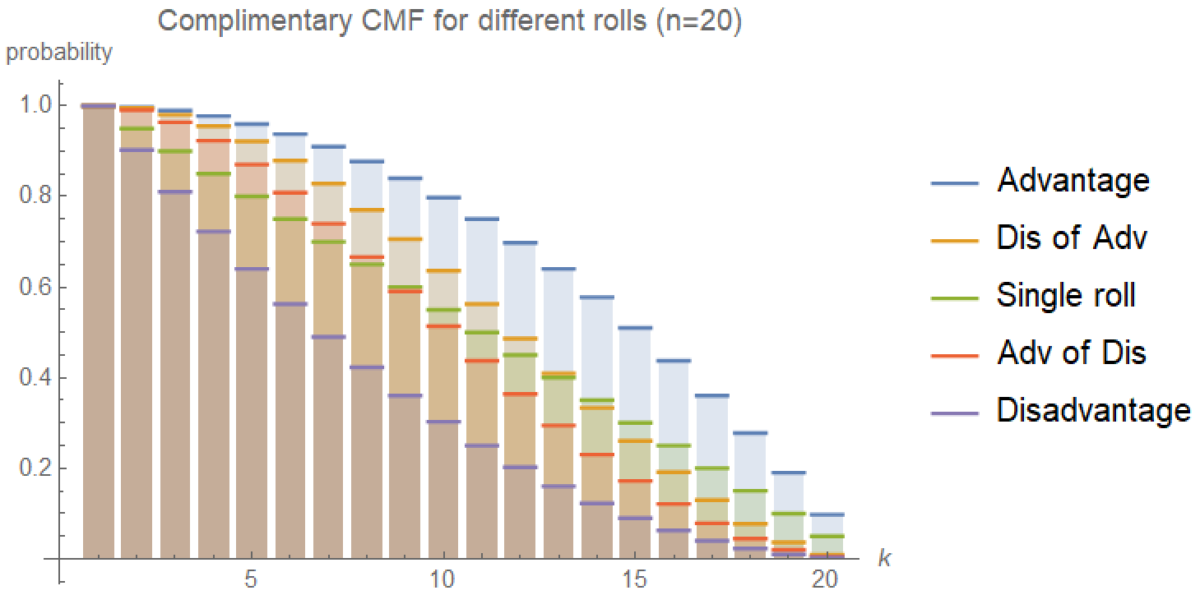
If the task is to roll $k$ or better, then we are seeking the probability that our outcome $X$ satisfies $X \ge k$. This is precisely the complimentary cumulative distribution function! Plotting these values for $n=6$, we obtain:

As anticipated, when $k=1$, all probabilities are $1$. The “advantage” roll is always best, while “disadvantage” is always worst. “disadvantage of advantage is second best for $k=1,2,3,4$, but for $k=5,6$ it’s best to roll a single die. We observe a similar result when $n=20$:

This time, “disadvantage of advantage” is second best for $1\le k \le 13$ and rolling a single die is best for $14 \le k \le 20$. In general, we can compute where the transition occurs as a function of $n$ by seeing which value of $k$ leads to $\bar F^{\text{DA}}_k = \bar F_k$. This leads to the equation:
\[
\frac{(n+k-1)^2 (n-k+1)^2}{n^4} = \frac{n-k+1}{n}
\]Solving this equation for $k$ and discarding extraneous solutions, we find the threshold occurs at:
\[
k_0 = 1 + \left( \frac{\sqrt{5}-1}{2} \right) n
\]So if $1\leq k < k0$, we have $\bar F^{\text{DA}}_k \gt \bar F_k$ and if $k_0 \lt k \leq n$, we have $\bar F^{\text{DA}}_k \lt \bar F_k$. Ok, so what happens in the limit? We can plot the continuous complimentary cdfs and obtain:

The pattern is the same, and we can solve for the cross-over point as before, by setting $\bar F^{\text{DA}}(z) = \bar F(z)$. This time, the equation is $(1-z^2)^2=1-z$. Solving for $z$, we obtain
\[
z_0 = \frac{\sqrt{5}-1}{2}
\]This is not surprising, as we could have simply normalized the discrete result as we did for expectations and take the limit $n\to\infty$ to obtain the same result. This number is the inverse of the Golden Ratio, neat!
I really like that using the continuous version, you were able to find the crossing point. It’s cute but curious that it’s 1/phi. Any intuition on why it should be?