Here is a puzzle from the
Riddler about gift cards:
You’ve won two gift cards, each loaded with 50 free drinks from your favorite coffee shop. The cards look identical, and because you’re not one for record-keeping, you randomly pick one of the cards to pay with each time you get a drink. One day, the clerk tells you that he can’t accept the card you presented to him because it doesn’t have any drink credits left on it.
What is the probability that the other card still has free drinks on it? How many free drinks can you expect are still available?
Here is my solution:
[Show Solution]
Let’s suppose each card starts with $n$ drinks. There are three ways the sequence of buying drinks can end:
- The first card gets maxed out and the second card has $k$ drinks remaining with $k\ge 1$. This means we purchased a total of $2n-k$ drinks and $n$ of them ended up on the first card. Then, we tried to purchase one additional drink on the first card and the buying stopped. The probability of this occurring is: $(\tfrac{1}{2})^{2n-k+1}\binom{2n-k}{n}$.
- both cards get maxed out and then we try to buy one more drink on either card. This means we purchased a total of $2n$ drinks and $n$ of them ended up on the first card. The probability of this occurring is $(\tfrac{1}{2})^{2n}\binom{2n}{n}$.
- The second card gets maxed out and the first card has $k$ drinks remaining with $k\ge 1$. This is exactly analogous to the first case, and the probability of this occurring is again: $(\tfrac{1}{2})^{2n-k+1}\binom{2n-k}{n}$.
Putting all of this together, we end up with a tidy formula for $p(n,k)$, the probability that when the game ends, the other card has exactly $k$ drinks remaining on it:
$\displaystyle
p(n,k) = \frac{1}{2^{2n-k}} \binom{2n-k}{n}
$
To double-check that this is a valid probability mass function, we should have $\sum_{k=0}^n p(n,k) = 1$. This is indeed the case, but it’s rather challenging to verify. Here is a link to the WolframAlpha computation. Here is plot of the probability mass function for $n=50$.

We can now answer the first question: the probability that the other card still has drinks on it is one minus the probability that there are no drinks left, i.e. $1-p(n,0)$. This evaluates to:
$\displaystyle
\mathrm{Prob}\Bigl(\begin{smallmatrix}\text{there are drinks left}\\\text{on the other card}\end{smallmatrix}\Bigr)
= 1-\frac{1}{4^n} \binom{2n}{n} \approx 1-\frac{1}{\sqrt{\pi n}}
$
This makes sense; the only way there can be no drinks left is if we purchased $2n$ drinks, and we were lucky to use each card exactly $n$ times. We would expect this probability to get smaller as $n$ gets larger. The approximation I used above comes from Stirling-like approximations for binomial coefficients (see here). When $n=50$ as in the problem statement, the probability evaluates to $92.04\%$. Here is a plot showing how the probability of there being drinks on the other card slowly tends to $1$ as $n$ gets larger:

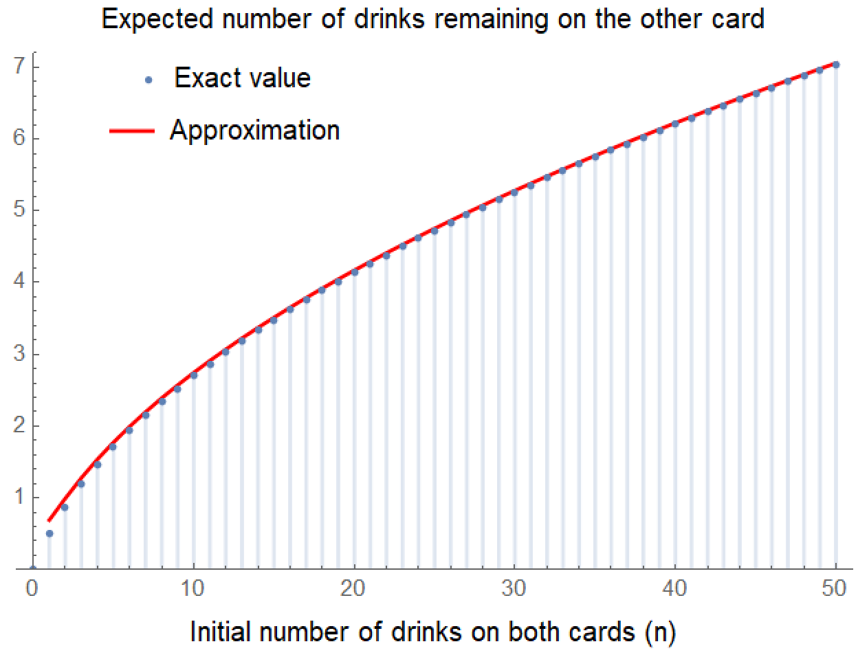
Now let’s address the second question: what is the expected number of drinks on the other card? We will compute the expected value directly from the probability mass function: $E_n = \sum_{k=0}^n k\, p(n,k)$. We find:
$\displaystyle
\mathbb{E}\Bigl(\begin{smallmatrix}\text{number of drinks left}\\\text{on the other card}\end{smallmatrix}\Bigr)
= \frac{2n+1}{4^n}\binom{2n}{n}-1 \approx \frac{2n+1}{\sqrt{\pi n}}-1
$
Again, the derivation is challenging so I omitted it, but here is the WolframAlpha link. Here is a plot of this function as it changes with $n$ along with the approximation (which is quite good!)

When $n=50$ as in the problem statement, the expected number of drinks remaining on the other card is $7.0385$. This corresponds to the expected value of the probability distribution plotted in the first image.


Nice. Glad to see the blog is back!
Another way to tackle this problem is, if people are familiar with absorbing state markov chains or Dirichlet boundary problems, consider the $m$ x $m$ matrix $\mathbf A$ that is all zeros, except all values are $0.5$ on its sub diagonal. This is a nilpotent matrix. We can construct the fundamental matrix then, of
$\mathbf N^{-1} = \mathbf A \oplus \mathbf A^T – \mathbf I_{m^2}$
where $\oplus$ denotes the Kronecker sum.
now solve for $\mathbf m$ in the equation
$\mathbf N^{-1}\mathbf m = \mathbf 1$
(where the RHS is the ones vector)
(A couple computational notes: there are typically optimized routines for solving linear equations involving Kronecker sums, though since the matrix isn’t symmetric, nothing came to mind. Not a problem in this exact case as the dimension isn’t too large, but things involving Kronecker products or sums get very big very quickly. Also of interest: this is a classic example of bad conditioning — all eigenvalues of $\mathbf N$ and its inverse are 1, but it’s a defective matrix, and more to the point the maximal singular value is quite far from one — again not an issue for this particular problem but it won’t scale very well)
At this point we’re basically done. The trick, that I misread at first, is that the ‘game’ doesn’t stop when one of the cards is at zero, it stops when a card is at zero and rejected — in effect this extends the game by 1. So select $m:= n+1 = 51$ for dimensions. Given monotone behavior in the markov chain, the maximal component value in $\mathbf m$ gives us the expected time until discovery — call this $\mu$.
But the value we want is expected residual life $\bar{X}$.
From here we need the identity that
$\mu + \bar{X} = 2\cdot m – 1$
(the identity should be straightforward application of linearity of expectations though there are some 0 vs 1 indexing nits to think through.)
Happy to post python code if anyone is interested.
– – – – –
The same method can in principle be used to recover the probability of both cards being empty at discovery time, but there are some more details involved and it gets rather messy to deal with I’m afraid.
A nicer way to get this value, which has echoes to the Problem of Points, is to consider this as a 2 player game– normally to get a nice distribution to work with, we’d extend the game to $2n – 1$ turns (this was the argument in Fermat’s approach). However, again, the game doesn’t end when someone is knocked out, but once they are discovered to be broke. So here we extend the game to $2n$ turns. If you look at the ‘real game’ vs the extended game, there is an exact correspondence in that in the real game, if someone ever has $n+1$ losses (i.e. discovered to be zero on that card) then even after playing more ‘filler games’ they still have $\geq n+1$ losses. So while we’ve transformed the probability distribution (and it is not appropriate to use this to get expected residual life on the other card), the probability of both being zero at discovery is maintained and it occurs iff $\binom{2n}{n}$ of the games are a ‘win’ for player a and the rest ‘wins’ for player b. Now we have a nice binomial (almost normal) distribution and the probability of this tie is given of course by $2^{-2n}\binom{2n}{n}$ — and the complementary probability gives the desired answer.
missed the edit cutoff. Some wordsmithing at the end of my post. Where I wrote
“occurs iff $\binom{2n}{n}$ of the games are a ‘win’ for player a and the rest ‘wins’ for player b”
it really should say instead:
occurs iff, exactly $n$ of the $2n$ games are a win for player a and the other $n$ are a win for $b$ — that is 2n choose n — i.e. $\binom{2n}{n}$.
– – – –
I also may have almost overloaded m. For clarification: the scalar $m$ just refers to dimension of matrix (i.e. an $\text{m x m}$ matrix). The vector $\mathbf m$ has components $m_i$ of course — but these don’t directly have anything to do with $m$. $\mathbf m$ is the mean time until absorption vector, with each component corresponding to a certain starting position. The way this is modeled, we want the ‘maximally far away’ starting position which is the one that fits the problem specifications. Obviously if we start at say 2 points left on card a and 3 points left on card b, then expected time until absorption will be less when starting with full cards.
here is some Python code to implement the above, for those interested. I switched to sparse matrices to speed this up quite a bit.
edit: I can’t get wordpress / markdown to respect this as code with associated whitespace. The good news is there are no whitespace adjustments needed, except that the line under the for loop needs indented. Everything else should run fine as is.
another edit: Aparently the rendered minus signs become dashes which also throws errors in python. Unfortunate that they must be hardkeyed over.
– – – – –
import numpy as np
from scipy.sparse import coo_matrix, kronsum
from scipy.sparse import identity as sparse_identity
from scipy.sparse.linalg import spsolve
m_dimension = 51 # needs an extra one adjustment
m = m_dimension
I = np.identity(m)
A = np.zeros((m,m))
for k in range(0, m_dimension-1):
A[k+1,k] = 1/2
A_sparse = coo_matrix(A)
L_sparse = sparse_identity(A.shape[0]**2) – kronsum(A_sparse, A_sparse.T)
result_sparse = spsolve(L_sparse, np.ones(m**2))
result_sparse_value = np.max(result_sparse)
print(2*m_dimension – 1 – result_sparse_value)
Yes, nice to have the blog back. It’s my go-to source for validating solutions without having to wait for the following Friday’s 538 post.
I suspected a nice analytical solution like this was possible, but I went ahead and hacked up a dynamic programming solution (and verified it with a Monte Carlo.)
My first thought on seeing the problem was that the probability of the other card still having value should be close to 1, and that the number of drinks left would also be close to 1. Then I wrote some code to simulate a few million iterations of coffee purchasing to see if these assumptions made sense. Output is below. 92% and 7+ both seemed off to me. At this point, confused as to how far both answers were from my sanity-check expectations, I switched over to other things I needed to get done and, basically, abandoned the problem. However, your math almost exactly matches my simulator output, so at least I have that going for me.
Output from simulating 1 million sets of coffee cards, run five times:
———
79850 of the 1000000 runs did not have any value left.
92.015% of the time the remaining card(s) have some value.
Mean Average remaining value is 7.6421692115416
79759 of the 1000000 runs did not have any value left.
92.0241% of the time the remaining card(s) have some value.
Mean Average remaining value is 7.63733630646755
79737 of the 1000000 runs did not have any value left.
92.0263% of the time the remaining card(s) have some value.
Mean Average remaining value is 7.64391483738888
79947 of the 1000000 runs did not have any value left.
92.0053% of the time the remaining card(s) have some value.
Mean Average remaining value is 7.6452367417964
79452 of the 1000000 runs did not have any value left.
92.0548% of the time the remaining card(s) have some value.
Mean Average remaining value is 7.65677400852536
Your intuition was correct — the probability that there are drinks left on the other card does tend to 1 as you increase the number of initial drinks. It just tends to 1 much more slowly than you might have expected. As I show, the probability is approximately $1-1/\sqrt{\pi n}$. So to get to 99%, for example, you need $n\gt 3183$.
Nice solution, Laurent! (I proposed the problem, and am glad you had fun with it!)
Your Stirling approximations are particularly impressive, and yours for the mean is different, and perhaps better, from that known: $2 \sqrt{N/\pi}-1$.
My path to the distribution is a little shorter, as follows.
Let’s first compute the probability that there are exactly $k$ drinks left on your other card. In this case, you used $100-k$ free drinks in total, and you used 50 from the declined card, distributed arbitrarily among the total. So, the probability is
$$
p(k) = { {100-k}\choose{50} } \left( 1 / 2 \right)^{100-k}
$$
The probability that there are still drinks left on the other card is $1-p(0) = 92$ percent. The expected value of this distribution over $k$ from 0 to 50 is about 7.
This can be obtained computationally or mathematically. Using a python program, it is 7.04. Using Stirling’s approximation, the expectation is approximately $2 \sqrt{50/\pi} – 1 = 6.98.$
Laurent,
Your approximation is indeed better than that known (at least to N = 133, the highest I tested).
An even better approximation is a linear combination of yours and the known one above:
$$\frac{ 2N+ \frac{e}{e+1} }{\sqrt{N \pi}} -1$$
For details, see
https://colab.research.google.com/drive/1Xh_dNckTURf2zUxZ94yjGxIKly68-FGf#scrollTo=InG8bEfXAFoQ