Assume you have a sport (let’s call it “baseball”) in which each team plays 162 games in a season. Assume you have a division of five teams (call it the “AL East”) where each team is of exact equal ability. Specifically, each team has a 50 percent chance of winning each game. What is the expected value of the number of wins for the team that finishes in first place?
The problem statement is a bit vague, so we must make some assumptions in order to solve the problem. Our first solution assumes that the win-loss records of the teams are mutually independent.
[Show Solution]
Our independence assumption basically reduces the AL East to a coin-flipping competition: each team flips 162 fair coins and counts the number of Heads obtained. The team with the most heads wins. In our second solution, we take a closer look at this assumption and discuss its validity.
Let’s say there are $m$ teams and each plays $n$ games. Let $Y_k$ be the number of wins obtained by team $k$. We’d like to find the average number of wins obtained by the team with the most wins. In other words, if we define $Y = \max(Y_1,\dots,Y_m)$, we would like to find $\mathbb{E}(Y)$. Note that multiple teams may be tied for first. If $p(y) = \mathbb{P}(Y=y)$ is the probability mass function, we may rewrite our quantity of interest using cumulative distributions (CDFs).
\begin{align}
\mathbb{E}(Y)
&= \sum_{y=0}^n y\, p(y)
= \sum_{y=0}^n \sum_{z=0}^{y-1} p(y)
= \sum_{z=0}^n \sum_{y=z+1}^n p(y) \\
&= \sum_{z=0}^n\left( 1 – \sum_{y=0}^z p(y)\right) \\
&= \sum_{z=0}^n\bigl( 1 – \mathbb{P}(Y \le z)\bigr)
\end{align}
Since $Y$ is the maximum over all $Y_k$, saying that $Y\le z$ is equivalent to $Y_k \le z$ holding for each $k$. Therefore:
\begin{align}
&= \sum_{z=0}^n\bigl( 1 – \mathbb{P}(Y_1 \le z, Y_2 \le z, \dots, Y_m \le z)\bigr) \\
&= \sum_{z=0}^n\bigl( 1 – \mathbb{P}(Y_1 \le z)\mathbb{P}(Y_2 \le z)\cdots\mathbb{P}(Y_m \le z)\bigr) \\
&= \sum_{z=0}^n\bigl( 1 – \mathbb{P}(Y_1 \le z)^m \bigr)
\end{align}
We made use of our independence assumption in the second equality, by stating that the joint cumulative distribution is equal to the product of cumulative distributions. In the third equality, we used the fact that each team has an identical win distribution, so each $\mathbb{P}(Y_k \le z)$ is the same for different $k$.
Since the games played by a particular team are assumed to be independent Bernoulli trials (coin-flips), the probability of a team winning $y$ of its $n$ games has a Binomial distribution with probability mass function $p(y) = {n \choose y} 2^{-n}$. Therefore, we have:
\[
\mathbb{E}(Y) = \sum_{z=0}^n\left( 1 \,-\, \frac{1}{2^{mn}} \left( \sum_{y=0}^z {n \choose y}\right)^m \right) = 88.3942…
\]
Unfortunately, there is no way to simplify the expression further, so the numerical answer you see above is what you get when you substitute $n=162$ games and $m=5$ teams. One can also use the fact that Binomial distributions approach Normal distributions when the number of trials is high. Namely, $B(n,p) \approx \mathcal{N}(np,np(1-p))$. Using this approximation,
\[
\mathbb{E}(Y) = \int_0^\infty \left[ 1 – \left(\frac{2}{n\pi}\right)^{\frac{m}{2}}
\left( \int_{-\infty}^x e^{-\frac{2}{n}\left(y-\frac{n}{2}\right)^2} \mathrm{d}y \right)^m \right] \mathrm{d}x \approx 88.4011
\]
It’s a pretty good approximation to our first solution, but unfortunately not much easier to evaluate! For the curious among you, here is what the distribution of wins of the best team looks like:

This next solution explains how to tackle the more realistic case where the games are not played independently, and explains why the independence assumption is a good one for the AL East.
[Show Solution]
The coin-flipping assumption we previously used allowed for the (unlikely) possibility of all five teams winning all their games. But this isn’t just unlikely, it’s impossible. In reality, some of the teams will play each other, so it’s impossible for every team to win every game. To illustrate this effect, let’s imaging a simpler scenario with only 3 teams, and each team plays 60 games. In the first plot, I use the independent coin-flip assumption. In the second plot, I assume the teams play each other exclusively.
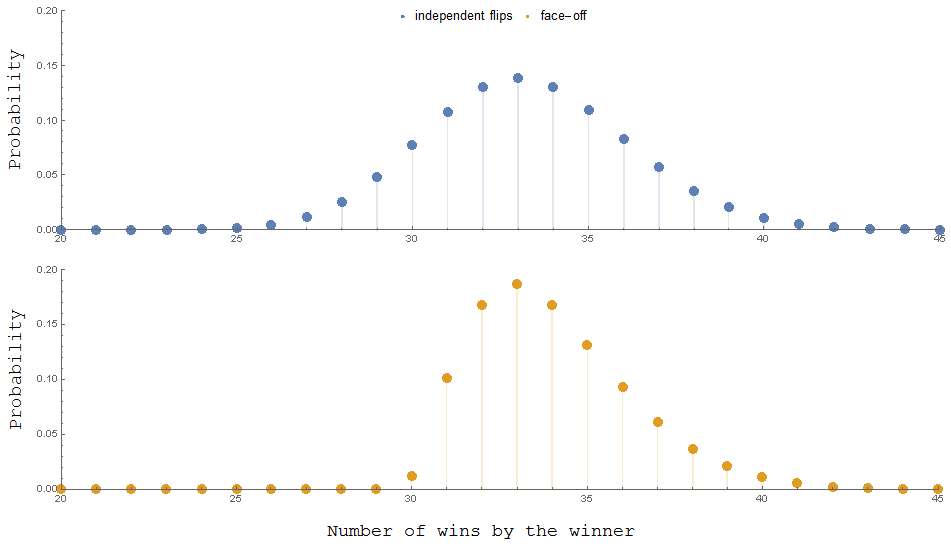
The most notable difference is that in independent case, it’s possible for a team to win the division despite only winning 29 of 60 games. This can’t happen when the teams play each other, since there will always be at least one team that wins at least half of their games. In the first plot, the expected value is $33.27$ while in the second plot it is $34.01$, a little bit larger. This effect diminishes as we add more teams, or if we have an intermediate scenario (e.g. some fraction of games are played within the division while others are treated as independent coin flips).
Will we see a significant effect in the AL East? In a typical 162-game season, each of the five AL East teams plays 19 games against each of the other four teams for a total of 76 games. Out of the remaining 86 games, 66 are against out-of-division opponents and 20 are against out-of-league opponents. It turns out that the additional teams together with the significant proportion of out-of-division games ends up drowning out the difference between both distributions. In other words, the assumption that each team simply flips 162 coins turns out to be a good one.
Here is one possible way to calculate the probabilities in the realistic case that accounts for inter-division games. Let’s suppose team $i$ plays team $j$ a total of $g$ times. Let $X_{ij}$ be the number of games team $i$ wins in that matchup. Then we clearly have $X_{ij} + X_{ji} = g$. Let $Z_i$ be the out-of-division wins acquired by team $i$. Then the total number of wins by each team in the AL East is:
\begin{align}
Y_k &= Z_k + \sum_{i\ne k} X_{ki} \\
&= Z_k + \sum_{i=1}^{k-1} X_{ki} + \sum_{i=k+1}^m X_{ki} \\
&= Z_k + \sum_{i=1}^{k-1} (g\, – X_{ik}) + \sum_{i=k+1}^m X_{ki} \\
\end{align}
So we have expressed $\{Y_1,\dots,Y_m\}$ (which are not independent) in terms of $\{X_{ij} \mid 1 \le i < j \le m\}$ and $\{Z_1,\dots,Z_m\}$, which are now independent. We’ll compute the CDF of the maximum of the $Y_k$’s as in the first solution. Using Bayes’ theorem,
\begin{align}
\mathbb{P}(Y \le z)
&= \mathbb{P}( Y_1 \le z,\dots, Y_m \le z ) \\
&= \mathbb{P}( Y_k \le z \mid X_{ij}, Y_k ) \prod_{i < j} \mathbb{P}(X_{ij}) \prod_{k=1}^m \mathbb{P}(Z_k)
\end{align}
Note that $X_{ij} \sim B(g,\tfrac12)$ and $Z_k \sim B(n-(m-1)g,\tfrac12)$ because each team plays $(m-1)g$ in-division games and so the remaining $n-(m-1)g$ games are out-of-division. Define the region:
\begin{align}
D &= \left\{ (x_{ij},z_k) \,\middle|\, 0 \le x_{ij} \le g,\quad 0 \le z_k \le n-(m-1)g \right\}\\
R(z) &= \left\{ (x_{ij},z_k) \,\middle|\, z_k + \sum_{i=0}^{k-1} (g\, – x_{ik}) + \sum_{i=k+1}^n x_{ki} \le z\,\,\forall k \right\}
\end{align}
So the distribution we seek is given by:
\begin{multline}
\mathbb{P}(Y \le z) \\
= \frac{1}{2^{m(n-\frac12 (m-1)g)}} \sum_{(x_{ij},z_k) \in D \cap R(z)} \prod_{i < j} {g \choose x_{ij}} \prod_{k = 1}^m {n – (m-1)g \choose z_k}
\end{multline}
The region $D\cap R(z)$ is simply a set of linear inequalities, so one could in principle evaluate the above sum. However, in the case of interest, $n=162$, $m=5$, and $g=19$, the sum has an astronomical number of terms, so some approximations are required to get an actual numerical answer in a reasonable amount of time. I’ll spare the details, but suffice to say that we obtain a distribution that is virtually identical to the one we found in the first solution. So the coin-flipping assumption turns out to be a good one for the AL East schedule!
I’d be curious to know, what’s the margin of error of the “independent coin tosses” simplification? You say we arrive at “a distribution that is virtually identical to the one we found in the first solution”, but what does that mean, numerically? Is there a simple way to approximate the error?
The final sum I obtained for the realistic solution has so many terms that it’s difficult (even for a computer) to evaluate it in a timely manner. So I used an integral approximation method similar to what I described in my first solution. Unfortunately, things don’t simplify as much as in the coin-flip case. You end up getting a pretty nasty integral that must again be approximated.
I computed and plotted a few sample points of the pmf and found that they coincided almost perfectly with the coin-flip points, so I decided not to put any more effort into getting an exact numerical answer.
So to answer your question, no — I don’t know of any simple way to approximate the error. Seems like you can either compute the approximate solution exactly (my first solution), or compute the exact solution approximately (my second solution)… and both give roughly the same answer!