In this interesting
Riddler problem, we’re dealing with a possibly unbounded sequence of… children? Here it goes:
As you may know, having one child, let alone many, is a lot of work. But Alice and Bob realized children require less of their parents’ time as they grow older. They figured out that the work involved in having a child equals one divided by the age of the child in years. (Yes, that means the work is infinite for a child right after they are born. That may be true.)
Anyhow, since having a new child is a lot of work, Alice and Bob don’t want to have another child until the total work required by all their other children is 1 or less. Suppose they have their first child at time T=0. When T=1, their only child is turns 1, so the work involved is 1, and so they have their second child. After roughly another 1.61 years, their children are roughly 1.61 and 2.61, the work required has dropped back down to 1, and so they have their third child. And so on.
(Feel free to ignore twins, deaths, the real-world inability to decide exactly when you have a child, and so on.)
Five questions: Does it make sense for Alice and Bob to have an infinite number of children? Does the time between kids increase as they have more and more kids? What can we say about when they have their Nth child — can we predict it with a formula? Does the size of their brood over time show asymptotic behavior? If so, what are its bounds?
Here is an explanation of my derivation:
[Show Solution]
Let’s call $t_k$ the time at which Alice and Bob have their $k^\text{th}$ child. The first child is born at time zero, so $t_1 = 0$. Since the work due to a child is one divided by their age, the work due to child $k$ at time $t$ is given by:
\[
\text{work at time }t = \begin{cases}
\frac{1}{t-t_k} & \text{if }t > t_k \\
0 & \text{otherwise}
\end{cases}
\]We also know that each new child is born once the total work due to all previous children equals $1$. Therefore, we have the following equations:
\begin{align}
t_2\text{ satsifies:} && \frac{1}{t_2-t_1} &= 1 \\
t_3\text{ satisfies:} && \frac{1}{t_3-t_2} + \frac{1}{t_3-t_1} &= 1 \\
t_4\text{ satisfies:} && \frac{1}{t_4-t_3} + \frac{1}{t_4-t_2} + \frac{1}{t_4-t_1} &= 1 \\
\cdots\qquad \\
t_k\text{ satisfies:} && \sum_{i=1}^{k-1} \frac{1}{t_k-t_i} &= 1
\end{align}and so on. We also know that $t_1 \lt t_2 \lt t_3 \lt \ldots$ since the children are born sequentially. The nice thing about these equation is that they can be solved sequentially. We know that $t_1=0$. Substituting this into the first equation yields $t_2=1$. Substituting these values into the second equation yields:
\[
\frac{1}{t_3-1}+\frac{1}{t_3} = 1
\]Rearranging yields $t_3^2-3t_3+1=0$. This equation has two solutions, but we take the one that satisfies $t_3 \gt t_2$, and we obtain $t_3=\tfrac{3+\sqrt{5}}{2} \approx 2.618$. We can continue in this fashion, solving each subsequent equation by substituting the previous values… but things get complicated in a hurry. The next equation becomes:
\[
t_4^3-\left(\tfrac{11+\sqrt{5}}{2}\right)t_4^2+\left(\tfrac{13+3\sqrt{5}}{2}\right)t_4-\left(\tfrac{3+\sqrt{5}}{2}\right)=0
\]Once again, we find that there is a unique solution that satisfies $t_4 \gt t_3$. This solution is approximately $t_4\approx 4.5993$. There doesn’t appear to be any automatic way to continue this process. Every time we try to compute the next $t_k$, we have to find the root of an even more complicated polynomial!
We’ll take a numerical approach, but let me first address one issue: how can we be sure that these ever-more-complicated polynomials always have a root that satisfies our constraints? For example, what if the polynomial for $t_4$ had no roots larger than $t_3$? What if it had many such roots? Thankfully, there is a simple way we can guarantee that there is always exactly one admissible root to each polynomial by leveraging the intermediate value theorem. Specifically, the function
\[
f_k(t) = \frac{1}{t-t_1} + \frac{1}{t-t_2} + \cdots + \frac{1}{t-t_{k-1}}
\]with $t \gt t_{k-1} \gt \ldots \gt t_1$ is a continuous and strictly decreasing function. Moreover, $\lim_{t\to {t_{k-1}}^+}f_k(t) = +\infty$ and $\lim_{t\to\infty} f_k(t) = 0$. Therefore, by the intermediate value theorem, there must be some point $t_k \in (t_{k-1},\infty)$ such that $f_k(t_k)=1$. The strict monoticity of $f_k$ ($f_k$ is strictly decreasing) implies that this $t_k$ must be unique.
The root may be unique, but how can we find it efficiently? Here, we can leverage a further property of $f_k$; namely convexity. The fact that $f_k$ is convex (and smooth) means that we can leverage some efficient methods from convex analysis that make use of derivative information. There are many ways to get the answer from here… What I ended up doing was to use the L-BFGS algorithm on the objective $(f_k(t)-1)^2$. My implementation in Julia using the Optim.jl package took about 40 seconds to evaluate birth dates of the first 1,000 children.
Note: there are many ways to formulate this as an optimization problem. One way is to note that solving $f_k(t)=1$ is equivalent to extremizing the antiderivative of $f_k(t)-1$. In other words, we could solve:
\[
t_k = \underset{t \gt t_{k-1}}{\text{arg min}} \left( t-\sum_{i=1}^{k-1}\log(t-t_i) \right)
= \underset{t \gt t_{k-1}}{\text{arg max}}\,\, e^{-t}\prod_{i=1}^{k-1}(t-t_i)
\]Incidentally, this last expression for $t_k$ makes it clear that there should be a unique $t_k$. When $t\gt t_{k-1}$, the product is a polynomial that is strictly increasing, and it’s multiplied by $e^{-t}$, which will drive it to zero eventually. There must therefore be a unique maximizer. I tried implementing both of these approaches and both turned out to be slower than directly minimizing $(f_k(t)-1)^2$.
If you’re just interested in the answers to the questions, here they are:
[Show Solution]
- Does it make sense for Alice and Bob to have an infinite number of children? Biological limitations aside, yes! We proved that for each $t_k$, there exists a unique $t_{k+1} \gt t_k$ that satisfies the constraints of the problem. So by induction, Alice and Bob can have as many children as they like.
- Does the time between kids increase as they have more and more kids? The answer is yes, and I will provide a “proof by picture”. After finding $t_k$ for $k=1,2,\dots$, we know the birth dates of each child. Then it remains to compute $(t_{k+1}-t_k)$ for each $k$ (the time between births). Here is the plot

The first point on the left says that we wait $1$ year after child $1$ is born, we wait about $1.6$ years after child $2$ is born, and so on. Plotted on a log scale as above, we see the curve is almost a perfect straight line. Here is a formula we can use to approximate the number of years to wait:
$\displaystyle
\text{years to wait after child }k\text{ is born} \,\approx\, 1 + 2.19\cdot \log_{10} k
$
So yes, the time between children increases (without bound), but it does so slowly. By the time Alice and Bob have their 1,000th child, they will be waiting approximately 7.5 years between kids.
- What can we say about when they have their $N^\text{th}$ child? Is there a formula we can write down? I couldn’t find an analytic expression, but I did find a pretty good approximation. First, let’s make a plot to see what we’re working with. Here is what the birth years is like for the first 19 children
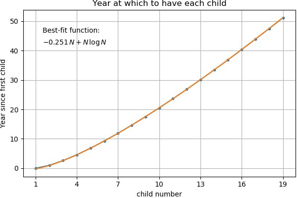
We can see here that the growth rate is slightly faster than linear. Since the time between children fit so well to a curve of the form $a+b\log x$, it makes sense to fit the birth dates themselves to the integral of this form. In an effort to fit the simplest possible curve, I did a bit of experimenting and found that the form $a x + x \log x$ does a really good job. I found the equation of best fit using linear regression and put the equation in the plot above. If we extend the time horizon, we get a similar result:

This is a pretty good fit; the plot actually depicts the true data with the fit overlaid on top. The fit is so good that you can’t even see the data underneath! So for large $N$, a good approximation is:
$\displaystyle
\text{year when child }N\text{ is born} \,\approx\,-0.315N + N\log N
$
- The final question is whether the size of the brood over time shows asymptotic behavior. We already plotted the time of birth vs child number, and found the relationship to be approximately: $y \approx -0.315 N + N\log N$. So here, we need to look at the inverse relationship and ask what $N$ does as a function of $y$. Since $y$ grows a little faster than linearly, this means $N$ will grow a little more slowly than linearly.
One thought: the problem solution structurally looks quite similar to what comes up in the derivation of Newton’s Identities, in particular
$\frac{p'(t)}{p(t)} = f_k(t) = \frac{1}{t-t_1} + \frac{1}{t-t_2} + \cdots + \frac{1}{t-t_{k-1}} =\sum_{i=1}^{k-1} \big(\frac{1}{t} + \frac{t_i}{t^2} + \frac{t_i^2}{t^3} + \cdots\big) = \frac{s_0}{t} + \frac{s_1}{t^2} + \frac{s_2}{t^3}+ \cdots$
where we have the power sum
$s_r := t_1^r + t_2^r + … + t_{k-1}^r$
(though in this case we are looking for the maximal $t$ that sets the above equal to one)
Nice observation — I thought about it a bit more and realized we could also express $t_k$ in the following compact form:
\[
t_k = \underset{t \gt t_{k-1}}{\text{arg max}}\,\, e^{-t}\prod_{i=1}^{k-1}(t-t_i)
\]It doesn’t buy us much, but it’s pretty! I updated my blog post to include this note.
Hi Laurent,
Very nice post, of course my results agree with yours.
I interpreted the question about “a formula” as a question “can I find an explicit expression” which you can for t1, t2 (linear equation), t3 (quadratic equation), t4 (cubic), and t5 (quartic), but there is no general formula for the roots of a quintic, so there is no “formula” for t6 (though there is an implicit relation or polynomial with instructions for root finding).
Regarding the asymptotic behavior, I think it’s not hard to show that
t_n – t_{n-1} = ln(n) + EulerGamma + O(1/ln(n))
and so far I think I calculated the O(1/ln(n)) term to be 1/( 4 ln(n)) + O(1/ln^2(n)).
The “proof” is that for large n, the spacing becomes nearly uniform. If it were precisely uniform, we would have (writing the spacing as Delta)
1 = 1/Delta + 1/(2 Delta) + … + 1/(n Delta) = (1/Delta) (ln(n)+EulerGamma+small)
resulting in Delta = ln(n) + EulerGamma.
Of course the spacing is not exactly uniform. Really we should write
1/(2 Delta) as 1/(Delta_n + Delta_{n-1}) and so forth.
But Delta_{n-1} is approximately EulerGamma + ln(n-1) = Delta – O(1/n). The sum of the 1/n corrections proves to be subleading by a 1/ln(n) factor….
very neat! thanks!
Guy, Laurent,
Thanks for your solutions/posts.
I used Guy’s insight to derive upper and lower bounds. The lower one turns out to be tight and close to Laurent’s line fit. (Laurent, this is with the -0.315N from your figure. Your text uses -3.15N. Is that a type?)
The upper bound diverges a bit but has a nice form.
See https://colab.research.google.com/drive/1fKSNWX3cZvbkx1XnWJDwXu3eDpgr_B4y#scrollTo=3iAgOeceH9BR or follow links from https://sites.google.com/view/msbits
I give a shout out to Guy’s comment and Laurent’s blog there. Please let me know if you would like me to provide alternate references.
Thanks! Yes that was a typo — I fixed it in the post.
Does the time between kids increase as they have more and more kids?
Proof by contradiction that the length of time between births increases without bound.
Let x_n be the length of time between the n-1 th and n th birthdays.
Assume there is a maximum length of time (y) between any two births.
The n+1 th birth will happen when:
1/x_n + 1/(x_n + x_n-1) + … + 1/(x_n + x_n-1 + … + x_2 + x_1) = 1
x_n <y
x_n + x_n-1 < 2y
…
x_n + x_n-1 + … + x_2 + x_1 < n y
1/y + 1/(2y) + 1/(3y) + … + 1/((n-1)y) + 1/(n y) < 1
1 + 1/2 + 1/3 + … + 1/(n-1) + 1/n < y
However, the sum on left hand side is the harmonic series which is known to diverge.
Therefore, the assumption is false and y (length of time between births) is unbounded with n.
Link to list of the first 10,000 birthdays:
https://docs.google.com/spreadsheets/d/1s5RtpjMd_RvCYDiw3TwQjlJUTOFX9CdSb46QBrPr_hw/edit?usp=sharing
I found a little different way to show asymptotic behavior. As you have stated
$$
\sum_{i=1}^{k-1}\frac{1}{t_{k}-t_{i}} = 1
$$
Rewrite this as
$$
\sum_{i=1}^{k-1}\frac{1}{1-\frac{t_{i}}{t_{k}}} = t_{k}
$$
For large $k$, if we posit a solution of the form
$$
t_{k} \simeq k H_{k-1}
$$
with $H_{k}$ being the Harmonic numbers, and noting that for large $k-i$,
$$
\frac{t_{i}}{t_{k}} \rightarrow 0
$$
and for small $k-i$
$$
\frac{t_{i}}{t_{k}} \rightarrow \frac{k}{k-i}
$$
you get the identity
$$
k H_{k-1} \simeq k \sum_{i=1}^{k-1} \frac{1}{k-i} = k H_{k-1}
$$
WOW This is nice!