 Roulette is a game where the dealer spins a numbered wheel containing a marble. Once the wheel settles, the marble lands on exactly one (winning) number. A standard American roulette wheel has 38 numbers on it. Players may place bets on a particular number, a color (red or black), or a particular quadrant of the wheel.
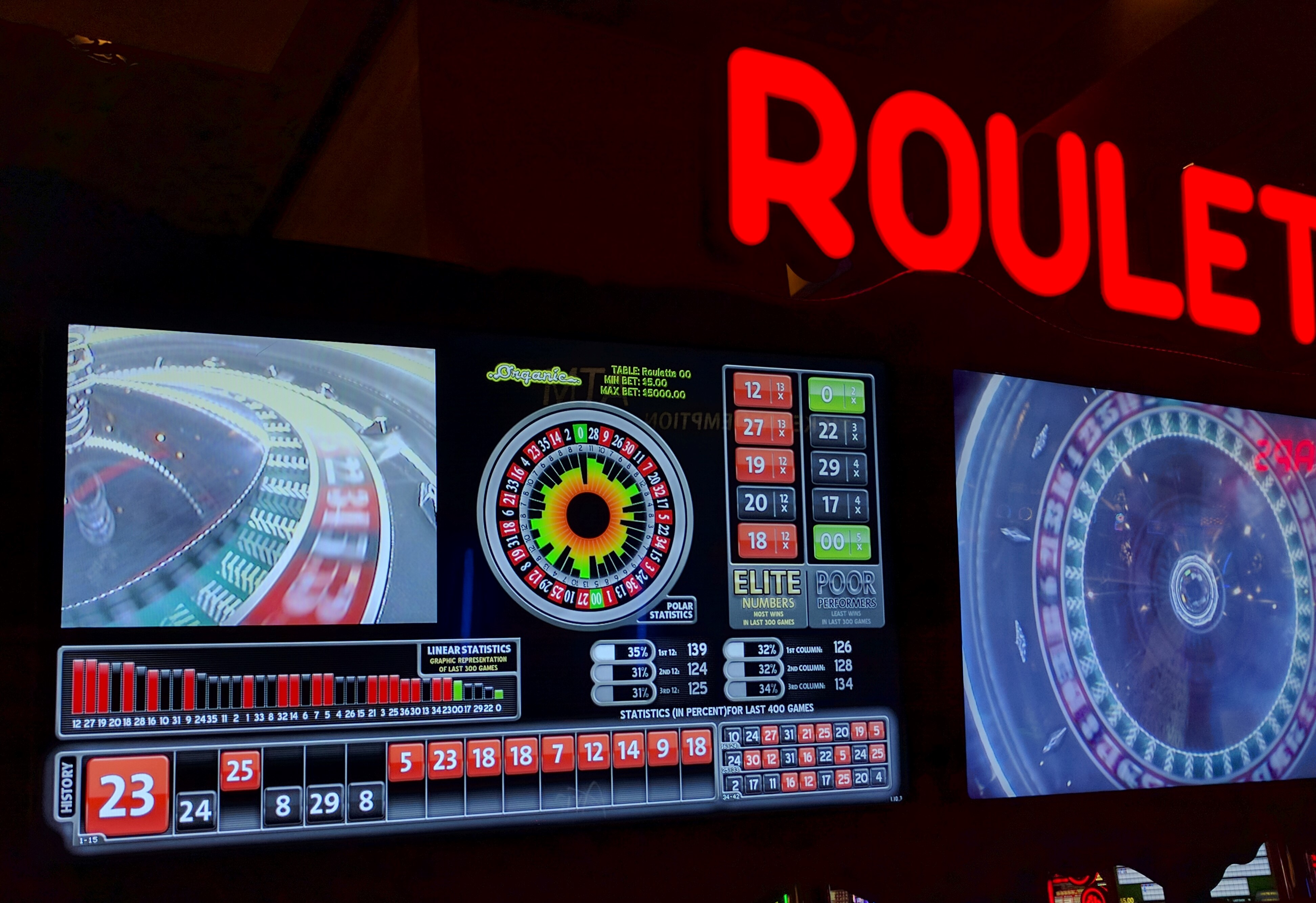
I was recently in Las Vegas for a conference, and I noticed that the roulette tables in the conference hotel were equipped with screens that display real-time statistics! A computer keeps track of the winning numbers for the past 300 spins and shows how frequently each number was a winner (see photo on the right). The two “elite numbers” were 12 and 27 (each occurred 13 times in the past 300 games) and the “poor performer” was 0, which only occurred 2 times.
Even if the roulette wheel is equally likely to land on each number, there will be natural fluctuations. Some numbers will obviously win more frequently than others in any finite number of spins. But what sorts of deviations can we expect? In the picture above, the spread between most frequent winner and least frequent winner was 13 to 2 over the course of 300 games. Is this normal? In other words, how big would the spread have to be before you suspected that the roulette wheel was rigged and was favoring some numbers over others? Let’s find out!
Results via simulation
Let’s suppose the wheel has $n$ different numbers on it, which we label $\{1,2,\dots,n\}$, and we spin it $m$ times when we aggregate our statistics. Note that in the actual roulette game, $n=38$ and $m=300$. If the game is fair, then each number is equally likely to occur and the spins are mutually independent. In other words, rolling a 4 on your first spin doesn’t make you more or less likely to roll a 4 or any other number on subsequent spins.
This sort of game is straightforward to simulate in Matlab. I wrote code that plays 300 games, counts how many times the most and least frequent numbers occur, and then repeats the entire process a large number of times. Then, I plotted a histogram showing what proportion of the time the most frequent number occurred 10 times, 11 times, etc. This is known as the empirical distribution. Here are the results of the simulation (aggregated over 100 million trials).

As we can see, a spread from 2 to 13 is right around what we expect! Of course, outliers are still possible. For example, it’s possible for the luckiest number to win 30 times out of 300 spins, but this only happened twice out of 100,000,000 simulated runs.
Analytical results
The roulette wheel lands on one of the $n$ numbers with equal probability. We then perform $m$ spins and count how many times each number occurs. If we place the counts in the vector $(x_1,\dots,x_n)$, where $x_1+\dots+x_n=m$, then this vector follows a multinomial distribution. The probability mass function is therefore:
\[
p(x_1,\dots,x_n) = {m \choose {x_1,\dots,x_m}} \frac{1}{n^m}
\]The bracketed term is called a multinomial coefficient and it counts the number of ways we can spin a “$1$” $x_1$ times, a “$2$” $x_2$ times, and so on. This also corresponds to the number of ways of depositing $m$ distinct objects into $n$ distinct bins, with $x_1$ objects in the first bin, $x_2$ objects in the second bin, and so on. It’s also equal to $\frac{m!}{x_1! \cdot x_2!\cdots x_n!}$. Meanwhile, $n^m$ is the number of different ways we can spin the roulette wheel $m$ times.
The probability that the most frequent spin occurs at most $k$ times is:
\[
F_\text{max}(k) = \sum_{\substack{ x_1+\dots+x_n=m\\x_i\,\le\,k}} p(x_1,\dots,x_n)
\]In other words, we must sum over all tuples $(x_1,\dots,x_n)$ of nonnegative integers that sum to $m$, that are each no greater than $k$. This is the cumulative distribution function, and in order to obtain the probability that the most frequent spin occurs exactly $k$ times (the probability mass function), we compute the difference:
\[
q_\text{max}(k) = F_\text{max}(k)-F_\text{max}(k-1)
\]A similar expression can be obtained for the probability that the least frequent spin occurs exactly $k$ times. These sums are impractical to compute because they have an astronomical number of terms. We must resort to approximation!
In our multinomial distribution, each $x_i$ has mean $\frac{m}{n}$ and variance $\frac{m}{n}\left(1-\frac{1}{n}\right)$. We will make the approximation that the $x_i$ are independent binomial random variables. Of course the $x_i$ are not truly independent since they must sum to $m$, but $n$ is large enough that this is a good approximation. We can therefore compute the distribution of the maximum by using the cumulative distribution:
\begin{align}
F_\text{max}(k) &= \mathbb{P}(x_1\le k,\dots,x_n\le k) \\
&\approx \prod_{i=1}^n \mathbb{P}(x_i \le k) \\
&= \left( \sum_{j=0}^k { m \choose j } \left( \frac{1}{n} \right)^j \left( 1-\frac{1}{n}\right)^{m-j} \right)^n
\end{align}This sum is far more manageable and we can compute it exactly without any difficulty. Once we have this cumulative distribution, we compute our approximation to $q_\text{max}(k)$ as before, by taking the difference of successive cumulative sums. The result is shown in the plot below.

As we can see, this plot is very close to the one we obtained via simulation. So the binomial approximation is quite good! It’s tempting to approximate the binomial distribution even further as a normal distribution, but it turns out this approximation isn’t very good. A rule of thumb to see whether we should use a normal distribution is to check whether 3 standard deviations of the mean keeps us within the range of admissible values, i.e. $\{0,1,\dots,m\}$. This amounts to checking, in our case, that $m > 9(n-1)$. Since $n=38$ and $m=300$, the inequality doesn’t hold because the right-hand side equals $333$.
Conclusion
Seeing one number occur 13 times while another only occurs 2 times in the past 300 spins isn’t abnormal at all. In fact, it’s very much what you should expect! So don’t think of the real-time statistics as a means to help you predict “lucky” or “unlucky” numbers… think of it as a way to double-check that the roulette wheel is unbiased!