A couple observations:
- when in any region of constant velocity (any of the smaller squares), the ant should move in a straight line, as this is the shortest (and therefore fastest) path between any two points.
- any shortest path must be reversible. If the ant were to retrace their steps and return to the start, they should be able to follow the same path back. This means our solution should have symmetry!
Let’s assume the speed is $1$ in the white squares and $\eta$ in the dark squares. It’s clear from the above that we can parameterize all paths through the board by one variable $x$, illustrated in the diagram below.

Since time is distance divided by speed, the time spent crossing the black squares is the distance divided by $\eta$. Meanwhile, the time spent crossing the white squares is just the distance (we assumed speed is 1 there). This makes the total time equal to:
\[
f(x) = \frac{2}{\eta}\sqrt{1+x^2} + \sqrt{2}\, (1-x)
\]Taking the derivative and setting it equal to zero, we find the optimal value of $x$ and the optimal associated time to be:
\[
x_\star = \frac{\eta }{\sqrt{2-\eta ^2}},\qquad
f(x_\star) = \sqrt{2}\left(1 + \frac{\sqrt{2-\eta^2}}{\eta}\right).
\]To answer the question asked, we should substitute $\eta=0.9$, and we find that $x \approx 0.825$ cm, and the time taken for the traverse is approximately $3.12835$ minutes.
Alternate derivation: Snell’s law!
It turns out this problem can be viewed through the lens (no pun intended) of optics! When a ray of light traverses an interface between two different media, it follows a path of least time.
This is known as Fermat’s principle of least time, and it leads to a formula in physics known as Snell’s Law: The ratio of the sines of the incidence angles is equal to the ratio of the velocities between the two media. In our case, illustrated below, the formula becomes
\[
\frac{\sin{\theta_1}}{\sin{\theta_2}} = \eta
\]

Based on the figure, we see that $\sin{\theta_1} = \frac{x}{\sqrt{1+x^2}}$ and $\sin{\theta_2} = \sin{\tfrac{\pi}{4}} = \frac{1}{\sqrt{2}}$. Therefore, Snell’s Law implies that
\[
\frac{x}{\sqrt{1+x^2}} = \frac{\eta}{\sqrt{2}}
\]Solving for $x$, we obtain the exact same formula we derived earlier!
Extra credit
Let’s consider a more general case, where the chessboard is $2n\times 2n$. The problem asks about the case $n=4$, but we will examine the general case. With the more complicated geometry, it’s not immediately clear what the path should look like, and where the crossings should occur. Nevertheless, we can make some logical deductions.
If we initially move to $(1,0)$ and then proceed diagonally in a straight line to $(2n,2n-1)$, the entire diagonal portion will be on white squares. Any path that travels farther than this diagonal will necessarily take more time and can be excluded. We therefore conclude that the entire path must be contained in the shaded region below.

In fact, the red region spans the range of all optimal paths for all $\eta$.
- When $\eta=1$, all squares have the same speed, so the fastest path is a straight line from start to finish (middle of the red region).
- When $\eta\to 0$, the black squares are significantly slower than the white ones, so we should minimize the time spent on black squares. This is done by moving along the boundary of the red region.
- When $0\lt\eta\lt 1$, the optimal path is somewhere in between!
By symmetry, we can further restrict the path to the lower half. We can see that for a $2n\times 2n$ square, there will be $4n-2$ interface crossings, and they will come in mirror-image pairs. This leaves $2n-1$ unknowns. We will label them as follows:

Due to the symmetry of the solution, the intersections occur in the order:
\[
x_1,x_2,\dots,x_{2n-1},x_{2n-1},\dots,x_2,x_1.
\]Finally, the total time is given by the expression:
\begin{multline}
f(x) = \frac{2}{\eta}\sqrt{1+x_1^2}+ \sqrt{2}\, \bigl(1-x_{2n-1}\bigr) \\
+ \sum_{k=0}^{n-2} \left( 2\sqrt{(1-x_{2k+1})^2+(1-x_{2k+2})^2}
+ \frac{2}{\eta}\sqrt{x_{2k+2}^2+x_{2k+3}^2}\right)
\end{multline}Note that when $n=1$ (the $2×2$ case from the first problem), the sums are empty and $x_1 = x_{2n-1}$ and we recover the $f(x)$ from the first part.
At this point, we must again take derivatives (gradients this time!) and set them all equal to zero, and solve the ensuing equations for $x_1,\dots,x_{2n-1}$. This is not a simple thing to do, and so I turned to Mathematica to find the solution numerically.
When $\eta=0.9$, the optimal time is approximately 11.78815 minutes, and the optimal crossings are:
\[
x_1 \approx 0.48571,\quad x_2 \approx 0.073789,\quad x_3 \approx 0.057876,\quad x_4=x_5=x_6=x_7=0.
\]So the last four crossings are zero. Zero?? Or just something really close to zero? This brings us to our bonus segment…
Phase transition madness!
We mentioned earlier that when $\eta\to 1$, the direct diagonal path is optimal, which means that $x_k \to 1$ for all $k$. Also, when $\eta \to 0$, the boundary of the red region is optimal, so $x_k \to 0$ for all $k$. So what happens for intermediate values of $\eta$? At first, I expected that all $x_k$ would gradually migrate from $0$ to $1$ as I increased $\eta$, but I was wrong!
What actually happens is that the $x_k$ stay exactly at $0$ until a certain $\eta$ threshold is crossed, at which point they move away from zero. Each different $x_k$ has a different $\eta$ threshold (!!)
Here is a plot of $x_1,\dots,x_7$ as functions of $\eta$ for the $8\times 8$ case.

So most of the $x_k$ are zero most of the time, until $\eta$ gets pretty close to $1$. Let’s zoom in to that interesting section of the plot:

So when $\eta=0.9$, only $x_1,x_2,x_3$ are nonzero, as we found earlier. But when $\eta=0.98$, all the $x_k$ are positive! The $\eta$ thresholds occur in pairs after $x_1$, i.e., $x_2,x_3$ become nonzero at the same time, so do $x_4,x_5$, and so on. This is because of how we defined the $x_k$. When $x_{2k}=0$, this forces $x_{2k+1}$ to be zero as well.
First remark: This phenomenon where varying a parameter can cause components of the optimal vector to go from zero to non-zero in a seemingly abrupt fashion also occurs in machine learning. Specifically, in L1-regularized least squares (Lasso regularization), as we vary the regularization parameter $\lambda$, the optimal vector $x$ transitions from sparse to dense with similar abrupt thresholds. The corresponding plot is called a regularization path.
Final remark: Although we only looked at the $8\times 8$ case, this plot actually tells us the solution for any value of $n$ (provided $\eta$ is not too large)! For example, suppose we wanted to solve the $500\times 500$ case with $\eta=0.96$. Based on our plot, we would simply read off the values of $x_1,\dots,x_5$ (they would be the same as in the $8\times 8$ case), and the remaining $x_k$ would be zero. The only caveat is that if we want to solve a case with $\eta \gt 0.97$ (which is larger than the threshold for $x_7$), then we would need to solve a larger grid such that we could find the missing thresholds.
Computing the first threshold analytically
Computing the exact values of $\eta$ at which the next $x_k$ becomes nonzero is not an easy task. With the help of Mathematica, I found that the first threshold occurs at the real root in $\eta \in (0,1)$ of
\[
117 \eta^8-576 \eta^6+1080 \eta^4-896 \eta^2+272=0
\]It turns out it has the exact value of:
\[
\eta_1 =
\sqrt{\frac{2}{39} \left(24-\sqrt{\alpha}-\sqrt{\frac{276}{\sqrt{\alpha}}-\alpha-27}\right)} \approx 0.885416,
\]where $\alpha := 13\cdot 3^{2/3}-9 \approx 18.0411$.
I tried computing $\eta_2$ as well, but it proved to be a lot more difficult!