Laurent - Book Proofs

Finding the doctored coin

This Riddler puzzle is about repeatedly flipping coins!

On the table in front of you are two coins. They look and feel identical, but you know one of them has been doctored. The fair coin comes up heads half the time while the doctored coin comes up heads 60 percent of the time. How many flips — you must flip both coins at once, one with each hand — would you need to give yourself a 95 percent chance of correctly identifying the doctored coin?

Extra credit: What if, instead of 60 percent, the doctored coin came up heads some P percent of the time? How does that affect the speed with which you can correctly detect it?

Here is my solution.
[Show Solution]

The first thing to realize about this problem is that the answer depends on how the coin flips turn out. For example, suppose that after $n$ flips, both coins came up heads an equal number of times. This is unlikely, but nonetheless it’s possible. We obviously can’t conclude anything about the coins in such a case. So the answer can’t depend only on $n$.

The coin flips are independent. So if a coin comes up heads with probability $p$ and we flip it $n$ times, the probability that it comes up heads exactly $k$ times is given by a Binomial distribution:
\[
B(n,p,k) = {n \choose k} p^k (1-p)^{n-k}
\]Let’s say the coins are numbered 1 and 2 and their probabilities of coming up heads are $p_1$ and $p_2$ respectively.

Now for the experiment: we flip each coin $n$ times and record how many times they come up heads (but we don’t know which coin is which). Let’s say they come up heads $k_1$ and $k_2$ times for the left and right coin respectively. Let’s call the data we observed $k$. There are two possible scenarios:

Coin 1 was in the left hand (and Coin 2 was in the right hand). We’ll call this scenario $\theta_1$. The likelihood of this scenario occurring is:
\[
\mathbb{P}(k\mid \theta_1) = B(n,p_1,k_1) B(n,p_2,k_2)
\]
Coin 1 was in the right hand (and Coin 2 was in the left hand). We’ll call this scenario $\theta_2$. The likelihood of this scenario occurring is:
\[
\mathbb{P}(k\mid \theta_2) = B(n,p_1,k_2) B(n,p_2,k_1)
\]

These are the only possible scenarios. If we want to be confident with level $\alpha$ about one of the scenarios then the posterior probability must be greater than $1-\alpha$. In other words:

If $\mathbb{P}(\theta_1\mid k) > 1-\alpha$, then we are confident in Scenario 1.
If $\mathbb{P}(\theta_2\mid k) > 1-\alpha$, then we are confident in Scenario 2.

Note that by definition, $\mathbb{P}(\theta_1\mid k)+\mathbb{P}(\theta_2\mid k) = 1$ for all $k$. So the two cases above can’t simultaneously be true when $\alpha\lt\tfrac{1}{2}$. We can compute posterior probability by using Bayes’ rule:
\[
\mathbb{P}(\theta_1\mid k) = \frac{\mathbb{P}(k\mid \theta_1)\mathbb{P}(\theta_1)}{\mathbb{P}(k\mid \theta_1)\mathbb{P}(\theta_1)+\mathbb{P}(k\mid \theta_2)\mathbb{P}(\theta_2)}
\]It is reasonable to assume that scenarios $\theta_1$ and $\theta_2$ have the same prior probability. So $\mathbb{P}(\theta_1)=\mathbb{P}(\theta_2)=\tfrac{1}{2}$. Therefore, our condition for confidence simplifies to:
\[
\frac{\mathbb{P}(k\mid \theta_1)}{\mathbb{P}(k\mid \theta_1)+\mathbb{P}(k\mid \theta_2)} > 1-\alpha
\quad\text{or}\quad
\frac{\mathbb{P}(k\mid \theta_2)}{\mathbb{P}(k\mid \theta_1)+\mathbb{P}(k\mid \theta_2)} > 1-\alpha
\]Rearranging these inequalities, we have:
\[
\frac{\mathbb{P}(k\mid \theta_1)}{\mathbb{P}(k\mid \theta_2)} > \frac{1-\alpha}{\alpha}
\quad\text{or}\quad
\frac{\mathbb{P}(k\mid \theta_2)}{\mathbb{P}(k\mid \theta_1)} > \frac{1-\alpha}{\alpha}
\]If we take logs of both sides, we can combine the expressions into a single inequality involving the difference of log-likelihoods, namely:
\[
\bigl|\, \log \mathbb{P}(k\mid \theta_1)-\log \mathbb{P}(k\mid \theta_2)\, \bigr| > \log\left(\tfrac{1}{\alpha}-1\right)
\]This has a nice interpretation: we can stop flipping coins once the difference between log-likelihoods grows sufficiently large. The smaller we make $\alpha$, the larger the difference in log-likelihoods must be before we can declare that we are confident.

We can simplify the expression considerably by substituting the definitions for the likelihoods $\mathbb{P}(k\mid \theta_1)$ and $\mathbb{P}(k\mid \theta_2)$ in terms of the $B(\cdot)$ functions, and substituting the binomial probability mass functions. Doing this, we obtain the simpler expression:
\[
|k_1-k_2| \left|\, \log \left( \tfrac{1}{p_1}-1 \right)-\log\left(\tfrac{1}{p_2}-1\right) \,\right| > \log\left(\tfrac{1}{\alpha}-1\right)
\]Note that $p_1$, $p_2$, $\alpha$ are parameters of the problem. The only part that change from case to case is $k_1$ and $k_2$. While it is customary to use a normal approximation when dealing with binomial distributions, doing so actually produces a more complicated formula, so we stick with binomials. The dependence on $n$ becomes evident if we express this formula in terms of the empirical probabilities $\hat p_1 := k_1/n$ and $\hat p_2 := k_2/n$. We obtain:

$\displaystyle
n \,>\, \frac{1}{|\hat p_1-\hat p_2|} \frac{\log\left(\frac{1}{\alpha}-1\right)}{\left|\, \log(\tfrac{1}{p_1}-1)-\log(\tfrac{1}{p_2}-1) \,\right|}
$

This is exactly the sort of expression we’re after — a lower bound on the number of samples required. This result agrees with our initial intuition: if $\hat p_1-\hat p_2 \to 0$, then $n\to \infty$. If the proportion of heads for both coins is the same, then we can’t possibly infer anything!

Expected solution. The number of flips required will be different depending on how the flips turn out. One way to get a numerical solution is to assume that the empirical probabilities match the true probabilities. In this case, we can substitute the values $\hat p_1 = p_1=0.5$, $\hat p_2 = p_2=0.6$, and $\alpha=0.05$ into the formula above, and we obtain $n \approx 73$.

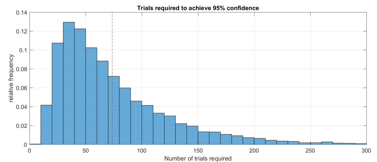
We can also simulate: generate random coin flips, compute empirical probabilities, and record how many flips were required to satisfy the 95% criterion. Then repeat many times and plot the distribution of stopping times. Here is what you get when you do this with 10,000 trials.

This distribution is very broad; sometimes only a dozen flips are required, other times over 300 flips are required. But the mean of the distribution (indicated in red) is close to our approximation of 73.

Varying the probability. We can also see what happens to the mean stopping time as we change the probability. Here, I assumed that $\hat p_1 = p_1 = 0.5$ and I plotted the average number of flips required to achieve 95% confidence as a function of $p_2$. Here is what I got:

As $p_2$ gets closer to $0.5$ (which is the value of $p_1$), it takes more and more flips to be able to tell the coins apart.

Sticks in the woods

This Riddler puzzle is about making triangles out of sticks! Here is the problem:

Here are four questions about finding sticks in the woods, breaking them, and making shapes:

If you break a stick in two places at random, forming three pieces, what is the probability of being able to form a triangle with the pieces?
If you select three sticks, each of random length (between 0 and 1), what is the probability of being able to form a triangle with them?
If you break a stick in two places at random, what is the probability of being able to form an acute triangle — where each angle is less than 90 degrees — with the pieces?
If you select three sticks, each of random length (between 0 and 1), what is the probability of being able to form an acute triangle with the sticks?

For the tl;dr, here are the answers:
[Show Solution]

Here are detailed solutions to all four problems (with cool visuals!):
[Show Solution]

Problem 1

Given three lengths $a,b,c$, when can they form a triangle? When they satisfy the triangle inequality! In other words, whenever:
\[
a+b > c
\quad\text{and}\quad
b+c > a
\quad\text{and}\quad
c+a > b
\]This makes sense when you think about it; if one of these inequalities were to be false, then one length would be longer than the sum of the other two, so no triangle would be possible.

Let’s say the stick has length 1, and it is broken at locations $a$ and $b$ (measured from the same side). We’ll assume that “broken at random” means that $a$ and $b$ are uniformly and independently distributed random variables on $[0,1]$. By symmetry, the cases $a\lt b$ and $b \lt a$ occur with equal probability and have the same probability of producing triangles, so let’s assume $a\lt b$. The three sidelengths are $(a, b-a, 1-b)$. Writing out the three triangle inequalities, we have:
\[
b > \tfrac{1}{2}
\quad\text{and}\quad
a < \tfrac{1}{2} \quad\text{and}\quad b-a < \tfrac{1}{2} \]Since $a$ and $b$ are uniform random variables, we can think of each $(a,b)$ as the coordinates of a point in the square $0 \le a \le 1$ and $0 \le b \le 1$. The probability we seek is precisely the area of the points satisfying our constraints. If we plot these points (and include the mirror case where $b \lt a$ as well), here is the figure we obtain:

We can see by inspection that the shaded area is $\tfrac{1}{4}$ of the total area. So the probability of forming a triangle by breaking a stick into three pieces is 25%.

Problem 2

In this version, we’re still trying to make a triangle, so we must enforce the same triangle inequalities as in Problem 1. In this version, however, we choose three sticks of lengths $a,b,c$ and each length is an independent random variable in the interval $[0,1]$. In this case, it is equally likely that $a$, $b$, or $c$ is largest. We’ll assume without loss of generality that $c$ is largest. In this case, we only need to worry about one of the triangle inequalities, so we have:
\[
a < c \quad\text{and}\quad b < c \quad\text{and}\quad c < a+b \] Here is what it looks like when we plot the first two inequalities (in pale yellow) and then the subset of that region that also satisfies the third inequality (in dark yellow).

It’s clear that the dark region has half the volume of the entire region, so the probability that the three pieces will form a triangle is $\tfrac{1}{2}$. We can also fill the rest of the cube by symmetry, and we obtain:

If you stare at this long enough, you realize that it’s just three identical copies of the previous region glued together (so the pale yellow is now the entire cube), so this shape again has half the volume of the entire cube. In summary, the probability of forming a triangle with three randomly chosen lengths is 50%.

Problem 3

Things start to get more complicated here. We’d like to make not just a triangle, but an acute triangle. This means that each interior angle must be less than 90 degrees. If the side lengths are $a,b,c$, we have from the law of cosines that $\cos(C) = \tfrac{a^2+b^2-c^2}{2ab}$ where $C$ is the angle opposite side $c$. If we want $0\le C \le \tfrac{\pi}{2}$, then we should choose $\cos(C)\ge 0$. This holds for all three angles, so we must have:
\[
a^2+b^2 > c^2
\quad\text{and}\quad
b^2+c^2 > a^2
\quad\text{and}\quad
c^2+a^2 > b^2
\]It turns out that these inequalities imply the triangle inequalities. Take the first one for example:
\[
c < \sqrt{a^2+b^2} < \sqrt{a^2+2ab+b^2} = a+b \]So we don't need to include the original triangle inequalities when we use these quadratic inequalities instead. Here is what the figure looks like when we plot all the inequalities and then mirror the image for the case $b\lt a$:

This is a much more complicated shape than what we had before. We’ll compute its area by computing the areas of the complementary pieces, pictured below:

Each of the four blue regions have equal area by symmetry. One of them is given by the inequalities:
\[
(1-b)^2 \ge (b-a)^2 + a^2
\quad\text{and}\quad
0 \le a \le \tfrac{1}{2}
\quad\text{and}\quad
b \ge \tfrac{1}{2}
\]Solving the first inequality for $b$, the boundary is given by: $b=\frac{1-2a^2}{2(1-a)}$. Therefore, we can compute one of the blue areas by evaluating the integral:
\[
A_\text{blue} = \int_{0}^{1/2} \left(\frac{1-2a^2}{2(1-a)}-\frac{1}{2}\right)\,\mathrm{d}a=\frac{3}{8}-\frac{1}{2}\log(2)
\]We can use a similar approach for each of the yellow regions, and we find:
\[
A_\text{yellow} = \int_{1/2}^{1} \frac{2a-1}{2a}\,\mathrm{d}a=\frac{1}{2}-\frac{1}{2}\log(2)
\]Putting everything together, we can calculate the area of the original blue shape, and it’s given by:
\begin{align}
A_\text{acute} &= \frac{1}{2}-4A_\text{blue}-2A_\text{yellow} \\
&= \frac{1}{2}-4\left(\frac{3}{8}-\frac{1}{2}\log(2)\right)-2\left(\frac{1}{2}-\frac{1}{2}\log(2)\right) \\
&= \log(8)-2 \approx 0.07944
\end{align}So the probability of forming an acute triangle by breaking a stick into three pieces is about 7.9%.

Problem 4

We’ll solve this problem the same way we solved Problem 2, but we’ll replace the triangle inequalities with the acute triangle inequalities used in Problem 3. As in Problem 2, we end up with a 3D volume rather than a 2D area. For simplicity again, we’ll assume that $c$ is the largest length, which accounts for one third of all possibilities. Here is the volume we get:

While this looks like a more complicated shape than the one from Problem 2, the curved surface has equation $c^2=a^2+b^2$, which is just the equation of a right circular cone! So we can calculate the volume of the region of interest by subtraction. It’s $1/3$ of the volume of the cube minus $1/4$ of the volume of the cone. The total probability is three times this volume, because we must account for the remaining identical pieces. The final answer is:
\[
P_\text{final}=3\left( \frac{1}{3}-\frac{1}{4}\left( \frac{\pi}{3} \right) \right) =1-\frac{\pi}{4} \approx 0.2146
\]So the probability of forming an acute triangle with three randomly chosen lengths is about 21.5%.

Just for fun, here is what you get when you put all three shapes together!

A tetrahedron puzzle

This post is about a 3D geometry Riddler puzzle involving spheres and tetrahedra! Here is the problem:

We want to create a new gift for fall, and we have a lot of spheres, of radius 1, left over from last year’s fidget sphere craze, and we’d like to sell them in sets of four. We also have a lot of extra tetrahedral packaging from last month’s Pyramid Fest. What’s the smallest tetrahedron into which we can pack four spheres?

Here is my solution:
[Show Solution]

We’ll solve this problem using old school (read: high school) geometry. Rather than starting with four spheres and looking for the smallest tetrahedron that contains them, we’ll solve the equivalent problem of starting with a fixed tetrahedron and looking for the largest spheres we can pack inside. We’ll use a tetrahedron of unit sidelength. Place one vertex at the origin $\vec O(0,0,0)$, one vertex on the $x$-axis $\vec P(1,0,0)$, and one face in the $xy$-plane. This leads to a vertex at $\vec Q(\frac{1}{2},\frac{\sqrt{3}}{2},0)$ because $OPQ$ is an equilateral triangle. To find the final vertex $R$, we know by symmetry that its $x$ and $y$ coordinates are the same as those of the centroid of $OPQ$, so $x=\frac{1}{2}$ and $y=\frac{\sqrt{3}}{6}$ (it’s at one third the altitude!). To find the final coordinate, we look for $z$ such that $x^2+y^2+z^2=1$, since all sides have length $1$. This leads us to the final vertex of the tetrahedron: $\vec R(\frac{1}{2},\frac{\sqrt{3}}{6},\frac{\sqrt{6}}{3})$.

The center of the tetrahedron can be found by looking for a point of the form $\alpha(\vec P+ \vec Q+\vec R)$ (again by symmetry) whose $x$-coordinate is $\frac{1}{2}$. Doing this leads us to the center: $\vec C(\frac{1}{2},\frac{\sqrt{3}}{6},\frac{\sqrt{6}}{12})$. Next, let’s look for the center of the sphere closest to the origin. By symmetry, it must be of the form $\vec C_1 = \beta \vec C$. We want to find $\beta$ such that it’s $x$-distance from the point $x=\frac{1}{2}$ is $r$ (so it just touches the sphere closest to $\vec P$), and we also want its $z$ coordinate to be $r$ (so it’s a distance $r$ from the $xy$ plane, because it’s a tangent point of the sphere). For a reference, see the figure below. I’m saying that $C_1$ (center of the sphere) should be on the line $OC$ and we should have $|C_1M| = |C_1A_1| = r$.

The equations just described are:
\begin{align}
\frac{1}{2} \beta &= \frac{1}{2}-r\\
\frac{\sqrt{6}}{12} \beta &= r
\end{align}
Solving this system of equations yields $\beta=\frac{6-\sqrt{6}}{5}$ and $r=\frac{\sqrt{6}-1}{10}\approx 0.145$. So this is the radius of the largest sphere we can use when the tetrahedron has sidelength $1$. If the radius is instead $1$, then we must scale the tetrahedron accordingly. The resulting sidelength will be:
\[
s = \frac{10}{\sqrt{6}-1} = 2\sqrt{6}+2 \approx 6.89898
\]Here is a scale diagram of the entire pyramid with the four spheres inside:

Is this bathroom occupied?

After a brief hiatus from Riddling, I’m back! This Riddler problem is about probability and bathroom vacancy.

There is a bathroom in your office building that has only one toilet. There is a small sign stuck to the outside of the door that you can slide from “Vacant” to “Occupied” so that no one else will try the door handle (theoretically) when you are inside. Unfortunately, people often forget to slide the sign to “Occupied” when entering, and they often forget to slide it to “Vacant” when exiting.

Assume that 1/3 of bathroom users don’t notice the sign upon entering or exiting. Therefore, whatever the sign reads before their visit, it still reads the same thing during and after their visit. Another 1/3 of the users notice the sign upon entering and make sure that it says “Occupied” as they enter. However, they forget to slide it to “Vacant” when they exit. The remaining 1/3 of the users are very conscientious: They make sure the sign reads “Occupied” when they enter, and then they slide it to “Vacant” when they exit. Finally, assume that the bathroom is occupied exactly half of the time, all day, every day.

Two questions about this workplace situation:

1. If you go to the bathroom and see that the sign on the door reads “Occupied,” what is the probability that the bathroom is actually occupied?
2. If the sign reads “Vacant,” what is the probability that the bathroom actually is vacant?
Extra credit: What happens as the percentage of conscientious bathroom users changes?

Here is how I solved the problem:
[Show Solution]

This problem can be solved using Bayes’ Rule but you can also use Markov chains. I like Markov chains so that’s what we’ll do!

The first step is to define what are states and transition probabilities are. This is the tricky part; we might be tempted to think that because the bathroom can be either occupied or not, and the sign in front can either read “Vacant” or “Occupied”, that there should be four states (one for each possible pair).

However, this is not the case. The reason is because the transition probabilities are not independent of one another. Consider the state “bathroom is occupied and the sign says it’s occupied”. We must distinguish between the cases where the person occupying the bathroom is conscientious (they will definitely slide the sign to “Vacant” when they leave) or not (they will leave the sign as “Occupied” after they leave).

We must therefore add additional states to our Markov chain that correspond to the different ways in which the bathroom can be occupied. To keep things general, let’s assume the fraction of oblivious, forgetful, and conscientious users are $p$, $q$, and $r$, respectively. Therefore $0\le p,q,r \le 1$ and $p+q+r=1$. A diagram of the Markov chain:

If $\{x_k\}$ denotes the probability of being in state $k$ in the diagram, the stationary distribution satisfies the equation:

\[
\begin{bmatrix}
0 & 0 & 1 & 1 & 0 & 0 \\
0 & 0 & 0 & 0 & 1 & 1 \\
p & 0 & 0 & 0 & 0 & 0 \\
r & r & 0 & 0 & 0 & 0 \\
q & q & 0 & 0 & 0 & 0 \\
0 & p & 0 & 0 & 0 & 0
\end{bmatrix}
\begin{bmatrix}
x_1 \\ x_2 \\ x_3 \\ x_4 \\ x_5 \\ x_6
\end{bmatrix}
=
\begin{bmatrix}
x_1 \\ x_2 \\ x_3 \\ x_4 \\ x_5 \\ x_6
\end{bmatrix}
\]

Solving these equations, we obtain:

\begin{align}
x_1 &= \frac{r}{2 (q+r)}, & x_2 &= \frac{q}{2 (q+r)}, & x_3 &= \frac{p r}{2 (q+r)}, \\
x_4 &= \frac{r}{2}, & x_5 &= \frac{q}{2}, & x_6 &= \frac{pq}{2 (q+r)}
\end{align}

We can now compute the probabilities we’re after:

\begin{align}
\mathbb{P}(\text{Vacant}\mid \text{says “Vacant”})
&= \frac{x_1}{x_1+x_3} = \frac{1}{1+p}\\
\mathbb{P}(\text{Occupied}\mid \text{says “Occupied”})
&= \frac{x_4+x_5+x_6}{x_2+x_4+x_5+x_6} = \frac{r+q-pr}{r+2q-pr}
\end{align}

When $p=q=r=\frac{1}{3}$ (equal fraction of conscientious, forgetful, and oblivious users), we obtain:
\begin{align}
\mathbb{P}(V\mid V) &= \frac{3}{4}, &
\mathbb{P}(O\mid O) &= \frac{5}{8}
\end{align}

Bonus: different probabilities

We have the analytic expressions above for what happens as a function of $p,q,r$… so now it remains to visualize it somehow. One possibility is to set two of them equal and just make a plot. For example, if we only vary the percentage of conscientious users ($r$) and set the other two to be equal, i.e. $p=q=\frac{1-r}{2}$. We then obtain:
\begin{align}
\mathbb{P}(V\mid V) &= \frac{2}{3-r}, &
\mathbb{P}(O\mid O) &= \frac{r^2+1}{r^2-r+2}
\end{align}We can also plot these probabilities as a function of $r$:

If we want to see what happens as we vary the percentages of $p,q,r$ all at once, we can visualize the result using a ternary density plot. Here, we plot values in a triangle; the fraction of each type of bathroom user is determined by the length of the altitude to the opposite side of the triangle and the color indicates the probability. Here are the plots:

You can read off the appropriate percentages by looking at the tick marks. For example, the lower-left corner corresponds to everybody being conscientious, the bottom (horizontal) side of the triangle corresponds to nobody being oblivious, and as you move from left to right you increase the fraction of forgetful users while simultaneously decreasing the fraction of conscientious users. The center of the triangle corresponds to $p=q=r=\tfrac{1}{3}$, and so on.

One additional comment: you’ll notice the point at the top of the triangle (100% oblivious users) is missing. This is because this probability doesn’t make sense. When all users are oblivious, the sign will never change. So if it starts at “Vacant”, it will stay at “Vacant” forever.

Squaring the square

This Riddler puzzle is about tiling a square using smaller squares.

You are handed a piece of paper containing the 13-by-13 square shown below, and you must divide it into some smaller square pieces. If you are only allowed to cut along the lines, what is the smallest number of squares you can divide this larger square into? (You could, for example, divide it into one 12-by-12 square and 25 one-by-one squares for a total of 26 squares, but you can do much better.)

Here is how I solved the problem:
[Show Solution]

This is a challenging puzzle and there is unfortunately no clever trick one can use to solve it quickly. If we consider the general problem of tiling an $N\times N$ grid using smaller squares, we can make several observations:

The smallest answer we could ever hope for is $4$. If $N=2k$ is even, we can achieve the minimum by splitting the square into four $k\times k$ squares. It’s clear that this solution cannot be improved.
If $N = 3k$ is a multiple of $3$, we can split it into six pieces: one $2k\times 2k$ square and five $k\times k$ squares. I believe this also cannot be improved.
When $N$ has many divisors, it becomes easier to tile it. The most challenging cases are therefore the cases where $N$ is prime. So a larger grid doesn’t necessarily mean a more difficult problem! We’ll see examples of this later.

I’ll solve this problem by converting it into an integer linear program (specifically, a variant of a knapsack problem), which can be solved much more efficiently than by brute-force checking the astronomical number of possible tilings.

I’ll illustrate the approach for the $5\times 5$ case. We’ll represent each possible square as a $5\times 5$ matrix of $0$’s and $1$’s. For example, we can use $25$ different $1\times 1$ tiles:
\[
\scriptsize \begin{bmatrix}{\color{red}{\color{red}1}}&0&0&0&0\\0&0&0&0&0\\0&0&0&0&0\\0&0&0&0&0\\0&0&0&0&0\end{bmatrix},
\begin{bmatrix}0&{\color{red}1}&0&0&0\\0&0&0&0&0\\0&0&0&0&0\\0&0&0&0&0\\0&0&0&0&0\end{bmatrix},
\begin{bmatrix}0&0&{\color{red}1}&0&0\\0&0&0&0&0\\0&0&0&0&0\\0&0&0&0&0\\0&0&0&0&0\end{bmatrix},\,\dots\,,
\begin{bmatrix}0&0&0&0&0\\0&0&0&0&0\\0&0&0&0&0\\0&0&0&0&0\\0&0&0&0&{\color{red}1}\end{bmatrix}
\]We can also use $16$ different $2\times 2$ tiles:
\[
\scriptsize \begin{bmatrix}{\color{red}1}&{\color{red}1}&0&0&0\\{\color{red}1}&{\color{red}1}&0&0&0\\0&0&0&0&0\\0&0&0&0&0\\0&0&0&0&0\end{bmatrix},
\begin{bmatrix}0&{\color{red}1}&{\color{red}1}&0&0\\0&{\color{red}1}&{\color{red}1}&0&0\\0&0&0&0&0\\0&0&0&0&0\\0&0&0&0&0\end{bmatrix},
\begin{bmatrix}0&0&{\color{red}1}&{\color{red}1}&0\\0&0&{\color{red}1}&{\color{red}1}&0\\0&0&0&0&0\\0&0&0&0&0\\0&0&0&0&0\end{bmatrix},\,\dots\,,
\begin{bmatrix}0&0&0&0&0\\0&0&0&0&0\\0&0&0&0&0\\0&0&0&{\color{red}1}&{\color{red}1}\\0&0&0&{\color{red}1}&{\color{red}1}\end{bmatrix}
\]Continuing in this fashion, we have $9$ different $3\times 3$ tiles and $4$ different $4\times 4$ tiles. So in total, we have $25+16+9+4=54$ different tiles. The name of the game is to pick the smallest possible subset of these matrices that sums to the matrix of all $1$’s. We can represent this compactly by vectorizing each of the $54$ matrices above into $25\times 1$ columns, and then stacking the columns side by side to form a matrix $A \in \{0,1\}^{25\times 54}$. Our goal is then to solve the problem:
\begin{align}
\underset{x \in \{0,1\}^{54}}{\text{minimize}}\qquad& \sum_{i=1}^{54} x_i \\
\text{subject to:}\qquad & Ax = 1
\end{align}Here, each $x_i$ is a binary variable that selects whether we’ll be using the $i^\text{th}$ column of $A$ or not. It turns out the optimal solution for this $5\times 5$ case uses $8$ squares; or the sum:
\begin{multline}
\scriptsize \begin{bmatrix}0&0&0&0&0\\0&0&0&0&0\\{\color{red}1}&{\color{red}1}&{\color{red}1}&0&0\\{\color{red}1}&{\color{red}1}&{\color{red}1}&0&0\\{\color{red}1}&{\color{red}1}&{\color{red}1}&0&0\end{bmatrix}
+\begin{bmatrix}{\color{red}1}&{\color{red}1}&0&0&0\\{\color{red}1}&{\color{red}1}&0&0&0\\0&0&0&0&0\\0&0&0&0&0\\0&0&0&0&0\end{bmatrix}
+\begin{bmatrix}0&0&0&{\color{red}1}&{\color{red}1}\\0&0&0&{\color{red}1}&{\color{red}1}\\0&0&0&0&0\\0&0&0&0&0\\0&0&0&0&0\end{bmatrix}
+\begin{bmatrix}0&0&0&0&0\\0&0&0&0&0\\0&0&0&0&0\\0&0&0&{\color{red}1}&{\color{red}1}\\0&0&0&{\color{red}1}&{\color{red}1}\end{bmatrix}\\
\scriptsize+\begin{bmatrix}0&0&{\color{red}1}&0&0\\0&0&0&0&0\\0&0&0&0&0\\0&0&0&0&0\\0&0&0&0&0\end{bmatrix}
+\begin{bmatrix}0&0&0&0&0\\0&0&{\color{red}1}&0&0\\0&0&0&0&0\\0&0&0&0&0\\0&0&0&0&0\end{bmatrix}
+\begin{bmatrix}0&0&0&0&0\\0&0&0&0&0\\0&0&0&{\color{red}1}&0\\0&0&0&0&0\\0&0&0&0&0\end{bmatrix}
+\begin{bmatrix}0&0&0&0&0\\0&0&0&0&0\\0&0&0&0&{\color{red}1}\\0&0&0&0&0\\0&0&0&0&0\end{bmatrix}
\end{multline}This general strategy of enumerating choices and then selecting among them doesn’t scale all that well because as $N$ gets large $A$ grows pretty quickly. In fact, $A$ will be $N^2 \times \tfrac{1}{6}(N-1)(2N^2+5N+6)$. However, in these cases we can use a heuristic such as column generation to quickly obtain approximate answers that can be iteratively and efficiently refined.

I solved the above integer linear program using Julia with JuMP and the Mosek solver. Read ahead for the results!

And here is the tl;dr, just the solutions!
[Show Solution]

The lucky derby

In the spirit of the Kentucky Derby, this Riddler puzzle is about a peculiar type of horse race.

The bugle sounds, and 20 horses make their way to the starting gate for the first annual Lucky Derby. These horses, all trained at the mysterious Riddler Stables, are special. Each second, every Riddler-trained horse takes one step. Each step is exactly one meter long. But what these horses exhibit in precision, they lack in sense of direction. Most of the time, their steps are forward (toward the finish line) but the rest of the time they are backward (away from the finish line). As an avid fan of the Lucky Derby, you’ve done exhaustive research on these 20 competitors. You know that Horse One goes forward 52 percent of the time, Horse Two 54 percent of the time, Horse Three 56 percent, and so on, up to the favorite filly, Horse Twenty, who steps forward 90 percent of the time. The horses’ steps are taken independently of one another, and the finish line is 200 meters from the starting gate.

Handicap this race and place your bets! In other words, what are the odds (a percentage is fine) that each horse wins?

Here is my full derivation (long!):
[Show Solution]

Let’s take a look at a particular horse. Each step, suppose it moves forward with probability $q > \frac{1}{2}$ or backward with probability $1-q$. The horse starts at position $0$ and we would like to know the probability that it will reach position $2n$ in exactly $2k$ steps. The reason for the factor of $2$ is that to reach an even-numbered position (such as $200$, in the problem statement), the horse must take an even number of steps. Let’s call this probability $P(n,k,q)$.

This scenario is known as a 1D random walk, and past posts that deal with similar ideas include The Deadly Board Game and Gambler’s Ruin. This problem is a bit different, however, since we care about the distributions of the number of moves required (not just the expected number of moves).

Back to the task at hand: determining $P(n,k,q)$. If we reach the position $2n$ in $2k$ moves, then clearly we have $k \ge n$. Next, we can deduce that we must have moved forward $(k+n)$ times and backward $(k-n)$ times. The probability of this occurring is $q^{n+k}(1-q)^{n-k}$. The tricky part here is to deal with the order in which we take the steps. The last step we take must always be forward, so we will restrict our attention to arrange the remaining $2k-1$ steps. There is a total of $2k-1 \choose k-n$ ways to do this, but this is not the number we’re looking for! Some of these paths will reach $2n$ too early, so we will count these paths and subtract them.

The quantity we’re counting is closely related to the Catalan Numbers, and we can borrow a similar proof technique (namely André’s reflection method) to arrive at the solution. Here is the argument: imagine the path laid out as a “mountain range” where each of the $2k-1$ steps is a move to the right and either up or down depending on whether the step was forward or backward. The diagram below illustrates a valid path for $n=2$ and $k=5$. Note that we are allowed to go negative!

We would like to exclude “bad paths” that reach $n$ at some earlier point. Consider the first point at which this occurs, and reflect the remainder of the path about the line $y=2n$. This leads to a new path that has $(k+n)$ forward steps, $(k-n-1)$ backward steps, and ends at $2n+1$ instead of $2n-1$. See the figure below for an illustration of the reflection method.

There is a one-to-one correspondence between bad paths and unconstrained paths of length $2k-1$ that reach $2n+1$. So the total number of valid paths (total paths minus bad paths) is given by:
\[
{2k-1 \choose k-n}-{2k-1 \choose k-n-1}=\frac{n}{k}{2k \choose k-n}
\]The simplification follows from (these identities), but can also be easily derived using algebra. Putting everything together, the probability of a horse first reaching $2n$ in exactly $2k$ steps is given by the formula:

$\displaystyle
P(n,k,q) = \frac{n}{k}{2k \choose k-n} q^{k+n} (1-q)^{k-n},\quad\text{for }k=n,n+1,\dots
$

We can plot the distributions for our case of interest, which is $n=100$ and $q$ varies from $0.52$ (for Horse $1$) up to $0.90$ (for Horse $20$). Here is a plot of the distributions for some of the horses:

As we can see, the distributions are normal to very good approximation. Although they are challenging expressions to manipulate, the task is not beyond the capabilities of Mathematica! In fact, we can verify that $P$ is a legitimate probability mass function and we can also compute its mean and variance for the case $\tfrac{1}{2} \lt q \le 1$:
\begin{align}
\sum_{k=n}^\infty P(n,k,q) &= 1 & & \text{(sums to 1)}\\
\sum_{k=n}^\infty k\, P(n,k,q) &= \tfrac{n}{2q-1} & & \text{(computing the mean)}\\
\sum_{k=n}^\infty \bigl(k-\tfrac{n}{2q-1}\bigr)^2 P(n,k,q) &= \tfrac{2nq(1-q)}{(2q-1)^3} & & \text{(computing the variance)}
\end{align}Here is the mean and standard deviation for a few of the horses:
\begin{align}
\text{Horse 4} &\approx 1250 \pm 218\\
\text{Horse 8} &\approx 625 \pm 74\\
\text{Horse 12} &\approx 417 \pm 37\\
\text{Horse 16} &\approx 313 \pm 21\\
\text{Horse 20} &\approx 250 \pm 12
\end{align}Note: we must double the means and standard deviations from the formulas above since those formulas skip over the odd lengths (which are impossible). When making a continuous approximation, we want those spaces filled in!

One thing we notice right away is that the distributions are very well separated (it’s a log scale!). The only horses that stand any chance of beating Horse 20 are the horses that are close behind. Let’s plot the distributions one more time, on a linear scale, but only for the top horses:

If horse $i$ finishes in $h_i$ steps, computing the probability that horse $i$ wins amounts to finding the probability that $h_i > h_j$ for all $i\ne j$. We can approximate this as:
\begin{align}
\mathbb{P}(h_i > h_j\,\,\forall i \ne j)
&\approx \int_{-\infty}^\infty \mathbb{P}(h_i = x) \prod_{j \ne i} \mathbb{P}(h_j > x)\, \mathrm{d} x\\
&= \int_{-\infty}^\infty \frac{1}{\sigma_i}\varphi_i(z_i)\prod_{j \ne i} \left( 1-\Phi(z_j)\right) \, \mathrm{d} x\\
\end{align}where $\varphi$ and $\Phi$ are the probability density (pdf) and cumulative distribution (cdf) of the standard Normal distribution and $z_k = \tfrac{x-\mu_k}{\sigma_k}$ is the standard normal deviate computed for the $k^\text{th}$ horse ($\mu_k$ and $\sigma_k$ are the mean and standard deviations computed earlier).

This is a very messy integral for which there does not exist a closed-form solution, so we must resort to evaluating it numerically. For the solution, read on!

For the tl;dr, the answer is:
[Show Solution]

Horse number	Probability of winning the race
20	71.27%
19	21.54%
18	5.605%
17	1.268%
16	0.2595%
15	0.05085%
14	0.01018%
13	0.002212%

Colorful balls puzzle

This Riddler puzzle about an interesting game involving picking colored balls out of a box. How long will the game last?

You play a game with four balls: One ball is red, one is blue, one is green and one is yellow. They are placed in a box. You draw a ball out of the box at random and note its color. Without replacing the first ball, you draw a second ball and then paint it to match the color of the first. Replace both balls, and repeat the process. The game ends when all four balls have become the same color. What is the expected number of turns to finish the game?

Extra credit: What if there are more balls and more colors?

Here is my solution to the first part (four balls):
[Show Solution]

Before I begin, I’d like to acknowledge Hector Pefo and Sawyer Tabony who also posted excellent solutions to this Riddler puzzle. We all arrived at the same answer (whew!) but our approaches differ slightly.

A natural way to think about this problem is that the game can exist in some number of states (the particular coloring of the balls in the box). At each step, at most one of the balls is recolored and we transition to another state. Such a collection of states and transition probabilities is known as a Markov Chain. Since we are only interested in how long it takes for all balls to be the same color, it’s not necessary to keep track of every possible state; we can aggregate states and simplify the problem.

Partition approach

One way to aggregate states is to count the number of balls of each different color without regard for the colors themselves. For example, 4 balls can be partitioned in 5 different ways:
\[
1+1+1+1,\qquad
2+1+1,\qquad
2+2,\qquad
3+1,\qquad
4
\]The partition “2+1+1”, for example, consists of cases where two of the balls are the same color and the other two balls are two other colors. Both the cases “red+red+green+blue” and “blue+blue+yellow+red” would fall into the category “2+1+1”. By using these five partitions as states in a Markov Chain, we can compute the transition probabilities to go from one state to the next. For example, the probability of transitioning from “2+1+1” to “3+1” is $\frac{1}{3}$ because in order for this transition to occur, we must first choose one of the two identically colored balls (probability $\frac{2}{4}$), then we must choose one of the other two balls out of the remaining three (probability $\frac{2}{3}$).

Here is what the complete Markov Chain looks like when all transition probabilities are filled in:

If we label the states in order, we can write the transition probabilities as a matrix that describes how states evolve.
\[
A = \begin{bmatrix}
0 & 0 & 0 & 0 & 0 \\
1 & \frac{1}{2} & 0 & 0 & 0 \\
0 & \frac{1}{6} & \frac{1}{3} & \frac{1}{4} & 0 \\
0 & \frac{1}{3} & \frac{2}{3} & \frac{1}{2} & 0 \\
0 & 0 & 0 & \frac{1}{4} & 0
\end{bmatrix}
\]For example, if $x$ is our current distribution, then $Ax$ is our distribution after one move. Note that the columns sum to $1$ because at each state, we must transition to some other state. The only exception is the last column, because the game stops once we reach the final state.

To compute the probability that the game ends after $k$ turns, we should find the probability that the game is in the final state after $k$ turns. Since we start in state $1$, the required quantity is $\left[ A^k \right]_{51}$. In other words, the $(5,1)$ component of $A^k$. We can compute this directly for each $k$ and we obtain the following distribution:

Note that the probability is zero for 1 or 2 turns because the game can’t end that quickly. It takes at least three turns (since there are four balls total) for all balls to be painted the same color. We can also compute the expected number of turns by evaluating the sum:
\[
A + 2A^2 + 3A^3 + \dots
= A(I-A)^{-2}
\]and then extracting the $(5,1)$ component. The result in this case turns out to be 9. When we compare the distribution to the mean in the figure above, we notice that the distribution has a heavy tail; although the mean is 9, the likeliest number of turns is actually 5.

Here is my solution to the general case with $N$ balls:
[Show Solution]

Although it’s possible to extend the partition used in the previous part to any other number of balls, in practice it is a challenge. One of the first obstacles is that the number of partitions as a function of $N$ is an intractable quantity. It is known as the partition function and is studied by number theorists for its deep connections to prime numbers. Partition functions were even mentioned in the recent movie about Ramanujan, “The Man Who Knew Infinity”. So we’re not taking that approach.

Counting Blue

We can still use Markov Chains, but we’ll have to come up with a different way of aggregating the states. One possibility is to define the states $k = 1,2,\dots,N$ which correspond to the number of Blue balls in the box. If Blue ends up winning, we will have started in state 1 and made our way eventually to state N without ever getting to state 0. The trick is to realize that no matter which color wins, the winning color has a Markov Chain like this one. All colors are indistinguishable so we might as well consider the case where Blue wins.

The next step is to compute transition probabilities. Here, we must be careful because we are conditioning on Blue winning. So we use Bayes’ Rule to compute the transitions. Given that there are $k$ Blue balls with $1 \le k \le N-1$, the probability that we transition $k\to k+1$ is:
\[
A_{k+1,k} = \frac{\mathbb{P}(k\to k+1 \text{, Blue wins})}{\mathbb{P}(\text{Blue wins})}
= \frac{\frac{k}{N}\cdot \frac{N-k}{N-1} \cdot \frac{k+1}{N}}{\frac{k}{N}} = \frac{(k+1)(N-k)}{N(N-1)}
\]Similarly, the probability that we transition $k\to k-1$ is:
\[
A_{k-1,k} = \frac{\mathbb{P}(k\to k-1 \text{, Blue wins})}{\mathbb{P}(\text{Blue wins})}
= \frac{\frac{N-k}{N}\cdot \frac{k}{N-1} \cdot \frac{k-1}{N}}{\frac{k}{N}} = \frac{(k-1)(N-k)}{N(N-1)}
\]The only other possibility is that we don’t transition at all, which is what happens the rest of the time. So $A_{k,k} = 1-A_{k+1,k}-A_{k-1,k}$. Simplifying the expressions, we obtain:
\[
A_{k+1,k} = \frac{(k+1)(N-k)}{N(N-1)},\quad
A_{k-1,k} = \frac{(k-1)(N-k)}{N(N-1)},\quad
A_{k,k} = 1-\frac{2k(N-k)}{N(N-1)}
\]As before, the $k^\text{th}$ column sums to 1. The only exception, as before, is the last column $A_{:,N}$, which is zero since the game ends once all colors are the same. The approach from here is identical to what we did when we used partitions. We can compute the probability of ending in $k$ turns by computing $\left[ A^k \right]_{N,1}$ and the expected number of turns is given by $\left[ A(I-A)^{-2} \right]_{N,1}$. Here are the distributions for $N=5$ and $N=8$.

As we can see, the distribution looks similar as we increase $N$. Curiously, the mean always appears to be $(N-1)^2$. In the next section, we will show that this is indeed the case in general!

Analytic expressions

Writing out the transition matrix explicitly, we have:
\[
A = \begin{bmatrix}
1-\frac{2(N-1)}{N(N-1)} & \frac{1(N-2)}{N(N-1)} & & & & 0 \\
\frac{2(N-1)}{N(N-1)} & 1-\frac{4(N-2)}{N(N-1)} & \frac{2(N-3)}{N(N-1)} & & & 0 \\
& \frac{3(N-2)}{N(N-1)} & 1-\frac{6(N-3)}{N(N-1)} & \ddots & & 0 \\
& & \frac{4(N-3)}{N(N-1)} & \ddots & \frac{(N-2)1}{N(N-1)} & 0 \\
& & & \ddots & 1-\frac{2(N-1)1}{N(N-1)} & 0 \\
& & & & \frac{N\cdot 1}{N(N-1)} & 0
\end{bmatrix}
\]If we define $a_k$ to be the expected number of turns until the game ends given that we are currently at state $k$, we can write the recursion:
\begin{align}
a_k &= 1 + A_{k+1,k} a_{k+1} + A_{k,k} a_k + A_{k-1,k} a_{k-1} \quad\text{for }k=1,\dots,N-1 \\
a_N &= 0
\end{align}Rearranging this expression, it looks roughly like $A^Ta+1=a$ (with the exception of the last row). Writing this as a single compact equation, we can factor things a bit and obtain a simpler equation:
\begin{multline}
\frac{1}{N(N-1)}
\begin{bmatrix}N-1 & & &\\ & \ddots & & \\ & & 2 & \\ & & & 1\end{bmatrix}
\begin{bmatrix}2 & -1 & & \\ -1 & 2 & \ddots & \\ & \ddots & \ddots & -1 \\ & & -1 & 2\end{bmatrix}\\
\times \begin{bmatrix}1 & & \\ & 2 & & \\ & & \ddots & \\ & & & N-1\end{bmatrix}
\begin{bmatrix}a_1 \\ a_2 \\ \vdots \\ a_{N-1}\end{bmatrix}
=
\begin{bmatrix}1 \\ 1 \\ \vdots \\ 1\end{bmatrix}
\end{multline}Or, simplified:
\[
\begin{bmatrix}2 & -1 & & \\ -1 & 2 & \ddots & \\ & \ddots & \ddots & -1 \\ & & -1 & 2\end{bmatrix}
\begin{bmatrix}a_1 \\ 2a_2 \\ \vdots \\ (N-1)a_{N-1}\end{bmatrix}
=
N(N-1)\begin{bmatrix}\frac{1}{N-1} \\ \frac{1}{N-2} \\ \vdots \\ 1\end{bmatrix}
\]By performing an LU decomposition, we may instead solve the following system of equations in sequence:
\begin{align}
\begin{bmatrix} 1 & & & & \\ -\frac{1}{2} & 1 & & & \\ & -\frac{2}{3} & 1 & & \\ & & \ddots & \ddots & \\ & & & -\frac{N-2}{N-1} & 1\end{bmatrix}
\begin{bmatrix} y_1 \\ y_2 \\ \vdots \\ y_{N-2} \\ y_{N-1} \end{bmatrix}
&= N(N-1)\begin{bmatrix}\frac{1}{N-1} \\ \frac{1}{N-2} \\ \vdots \\ \frac{1}{2} \\ 1\end{bmatrix}\\
\begin{bmatrix} 2 & -1 & & & \\ & \frac{3}{2} & -1 & & \\ & & \frac{4}{3} & \ddots & \\ & & & \ddots & -1 \\ & & & & \frac{N}{N-1} \end{bmatrix}
\begin{bmatrix} a_1 \\ 2a_2 \\ \vdots \\ (N-2)a_{N-2} \\ (N-1)a_{N-1} \end{bmatrix}
&= \begin{bmatrix}y_1 \\ y_2 \\ \vdots \\ y_{N-2} \\ y_{N-1}\end{bmatrix}
\end{align}The first system is easily solved for $y$ by forward-substitution. We first have $y_1=N$. Then, $y_2 = \frac{N(N-1)}{N-2}+\frac{1}{2}y_1$, and so on. The result we find is:
\[
y_k = N(N-1)\sum_{i=1}^k \frac{i}{(N-i)k}
\]The second system can be solved for $a$ by back-subsitution, starting from the final equation and working our way back up. Doing this, we find:
\[
a_k = \sum_{j=1}^{N-k} \frac{1}{k+j} y_{k+j-1}
\]We may now combine both expressions and obtain:
\[
a_k = N(N-1) \sum_{j=1}^{N-k} \frac{1}{k+j} \sum_{i=1}^{k+j-1} \frac{i}{(N-i)(k+j-1)}
\]This is a bit messy, but we only care about $k=1$ (the expected number of turns given that we start with only one blue ball and blue ends up winning). This sum can be simplified with a bit of work:
\begin{align}
a_1 &= N(N-1) \sum_{j=1}^{N-1} \frac{1}{j(j+1)} \sum_{i=1}^{j} \frac{i}{(N-i)} \\
&= N(N-1) \sum_{j=1}^{N-1} \left( \frac{1}{j}-\frac{1}{j+1}\right) \sum_{i=1}^{j} \frac{i}{(N-i)}
\end{align}Define $Q_j := \frac{1}{j+1}\sum_{i=1}^j \frac{i}{N-i}$ and the sum telescopes:
\begin{align}
a_1 &= N(N-1)\sum_{j=1}^{N-1} \left( \frac{1}{N-j} + Q_{j-1}-Q_j\right)\\
&= N(N-1)\left( \sum_{j=1}^{N-1}\frac{1}{N-j}-Q_{N-1} \right) \\
&= N(N-1)\left( \sum_{j=1}^{N-1}\frac{1}{N-j}-\frac{1}{N}\sum_{j=1}^{N-1}\frac{j}{N-j} \right) \\
&= N(N-1) \sum_{j=1}^{N-1}\frac{1}{N} \\
&= (N-1)^2
\end{align}And this is precisely what we were trying to show! The expected number of turns for a game with $N$ balls is $(N-1)^2$. A similar expansion can be done to compute $a_k$ for $k\ne 1$ but in this case there is only partial telescoping and we are left with
\[
a_k = (N-1)^2-\frac{N(N-1)}{k}\sum_{i=1}^k \frac{k-i}{N-i}
\]As $N$ gets large, the sum of reciprocals is well-approximated by a logarithm. If we denote $\alpha = k/N$ the fraction of balls that are blue, then the expected number of turns until all balls are blue is:
\[
\frac{a_k}{(N-1)^2} \approx \left(\frac{1-\alpha}{\alpha}\right)\log\left(\frac{1}{1-\alpha}\right)
\]Here is a scaled plot of this distribution of expected number of turns:

A conjecture?

I was intrigued by the distribution of the number of turns rather than just the expected value. As seen in the plots above, the distribution converges to something, but it’s not clear what. And there doesn’t appear to be an easy way to compute or approximate powers of $A$ analytically. I suspect the distribution tends to a log-normal distribution as $N$ gets large because when plotted on a log scale, it sure looks close to normal:

If you have any thoughts, leave a comment below!

Pick a card!

This Riddler puzzle is about a card game where the goal is to find the largest card.

From a shuffled deck of 100 cards that are numbered 1 to 100, you are dealt 10 cards face down. You turn the cards over one by one. After each card, you must decide whether to end the game. If you end the game on the highest card in the hand you were dealt, you win; otherwise, you lose.

What is the strategy that optimizes your chances of winning? How does the strategy change as the sizes of the deck and the hand are changed?

Here is my solution:
[Show Solution]

Approximate solution

Let’s suppose that the deck has $n$ cards in it, and we are dealt $k$ cards from the deck. Every time a card is flipped, we must decide whether to keep playing or to stop. Suppose we have flipped over $m$ cards already and the largest card flipped so far has a value of $a$. Some quick observations:

If the last card we flipped has value smaller than $a$, then we must clearly keep flipping cards, for we would definitely lose if we stopped playing now.
Assuming the last card we flipped has the largest value ($a$), we must evaluate the probability that the remaining $k-m$ cards are each smaller than $a$ (in other words, the probability that $a$ is the winner). We should compare this probability to the probability that we will win if we continue playing. Whichever is highest will dictate the optimal course of action.

One possible decision heuristic is to stop if the probability that the current card is a winner is greater than $1/2$ and to keep playing otherwise. This turns out to be a suboptimal strategy because our chances of winning might be even less if we keep playing! In other words, it could happen that we have a 49% chance of winning if we stop now but only a 45% chance of winning if we keep playing; in such a case, we should stop now and cut our losses. That being said, this suboptimal strategy is a very good approximation to the optimal strategy (and very easy to compute!) so let’s work it out.

Each of the $m$ cards we’ve flipped over so far is distinct and less than or equal to $a$. If the current card $a$ is the winner, then the remaining $k-m$ cards must all be chosen among the $a-m$ cards that are less than or equal to $a$. This can be done in $a-m \choose k-m$ ways. In total, there are $n-m \choose k-m$ ways of choosing the remaining cards. Therefore, we should stop playing if
\[
\frac{a-m \choose k-m}{n-m \choose k-m} \ge \frac{1}{2}
\]Clearly, this will be satisfied for $a$ sufficiently large, so our optimal decision rule is a threshold rule. There is no closed-form expression for the threshold value of $a$, but it’s straightforward to compute numerically. Here is a plot of the approximate decision rule for the case $n=100$, $k=10$.

The triangular white region in the lower corner corresponds to the case $a < m$, which can't occur because $a$ must be the largest number seen so far and all numbers must be distinct.

Exact solution

To get an exact solution, we’ll use dynamic programming. Let the cards be numbered $\{1,2,\dots,n\}$ and let $k$ be the number of face-down cards at the start of the game. In general, one might expect an optimal strategy to depend on the individual values of all the cards revealed thus far. This is not the case. It turns out that the optimal strategy only depends on:

How many cards we’ve seen so far (we’ll call this $m$)
The highest-valued card we’ve seen so far (we’ll call this $a$)
Whether the last card turned over is the largest so far or not.

We’ll define two functions, $V^\text{lo}_m(a)$ and $V^\text{hi}_m(a)$, to record the probability of winning the game in the case where the latest card we turned over is low or high, respectively.

Base case: Suppose $m=k$, so we have just flipped over the final card. The game automatically ends and we have no decisions to make. We win if the card we flipped over is the highest numbered card. In other words:
\[
\begin{aligned}
V^\text{lo}_k(a) &= 0 \\
V^\text{hi}_k(a) &= 1
\end{aligned}\qquad\text{for }a = 1,\dots,n
\]

Recursion: Now suppose that we’re $m$ steps into the game. Let’s start with the case of a low flipped card. Here, we’ll lose for sure if we stop the game. So we must keep playing. We’ll assume $y \in S$ is the next card we flip over. Here, $S \subseteq \{1,\dots,n\}$ is the set of cards we haven’t seen yet. Note that $|S| = n-m$ because we have flipped over $m$ cards so far. Any of these $n-m$ remaining cards could be flipped over next with equal probability. Let’s treat the cases $y < a$ and $y > a$ separately:
\begin{align}
V^\text{lo}_m(a) &= \frac{1}{n-m}\biggl( \sum_{y\in S,\,y < a} V^\text{lo}_{m+1}(a) + \sum_{y\in S,\,y > a} V^\text{hi}_{m+1}(y) \biggr) \\
&= \frac{1}{n-m}\biggl( (a-m) V^\text{lo}_{m+1}(a) + \sum_{y=a+1}^n V^\text{hi}_{m+1}(y) \biggr)
\end{align}In the last step, we use the fact that there are precisely $a-m$ terms in $V^\text{lo}$ sum, which doesn’t depend on $y$. In the $V^\text{hi}$ sum, we’re summing over all values larger than $a$, and no such values have been used yet.

For the case of a high flipped card, we can choose to either stop the game or keep playing. If we stop the game, we will win if the remaining $k-m$ cards all happen to be smaller than $a$, our current high card. There are $a-m$ cards that satisfy this property and $n-m$ cards left total, so the probability of winning is ${a-m \choose k-m}/{n-m \choose k-m}$. If we decide to keep playing instead, we get the same answer as in the low case. Therefore, our recursion is:
\[
V^\text{hi}_m(a) = \max\biggl\{ \underbrace{\frac{{a-m \choose k-m}}{{n-m \choose k-m}}}_{\text{STOP}}, \,
\underbrace{V^\text{lo}_m(a)}_{\text{PLAY}} \biggr\}\qquad\text{for }a=1,\dots,n
\]At this point, it’s not possible to proceed any further without resorting to numerical computations. The good news is that these recursions are relatively easy to tabulate numerically; we can store all relevant probabilities in two matrices $V^\text{lo},V^\text{hi} \in \mathbb{R}^{k\times n}$ and we can compute everything in $\mathcal{O}(n^2k)$.

Here is a plot of the optimal decision rule for the case $n=100$, $k=10$.

As we can see, this plot is very similar to the approximate rule. Here is a table of the threshold values for comparison:

Cards flipped	Approximate Threshold	Optimal Threshold
1	93	93
2	93	92
3	92	91
4	90	89
5	88	87
6	86	84
7	82	80
8	74	72
9	55	55
10	10	10

This means that e.g. if our ninth card is $55$ or greater, we should stop playing. Note that if we make it to the 10th turn and our final flipped card is still a contender (i.e. the largest we’ve seen so far), then that card cannot have a value less than $10$ and we automatically win.

Probability of winning

So how do we compute the actual probability of winning? We already have! If we have recursed all the way to $m=1$, then $V^\text{hi}_1(b)$ tells us the probability of winning given that the first card we flipped over was $b$ (and, of course, it was our highest card). Since all cards are equally likely first cards, we have:

$\displaystyle
\mathbb{P}(\text{winning}) = \frac{1}{n}\sum_{b=1}^n V_1^\text{hi}(b) = V_0^\text{hi}(1)
$

For the case $n=100$ and $k=10$, the probability of winning is 62.19%.

Limiting cases

We can easily compute what happens if we add more cards. Let’s fix $k=10$ and try $n=1000$.

As we can see, things don’t look that much different as we make $n$ large. We can approximate this limiting shape by taking the limit $n\to\infty$ while holding $a$ as some fixed fraction of $n$ and using our approximate strategy instead of the optimal one:
\begin{align}
\frac{a-m \choose k-m}{n-m \choose k-m}
= \prod_{j=1}^{k-m} \frac{a-m+1-j}{n-m+1-j}
\approx \prod_{j=1}^{k-m} \frac{a}{n}
= \left(\frac{a}{n}\right)^{k-m}
\end{align}Therefore the threshold (when this probability hits $1/2$) occurs when:
\[
a \approx n\,2^{-\frac{1}{k-m}}
\]We can overlay the limiting case formula with the actual one to see how well they match. Here is an example with $n=10000$ and $k=40$:

It’s a pretty good fit, with the thresholds for the optimal strategy being slightly lower than the optimal ones. Increasing $k$ is also straightforward, and simply amounts to shifting the above pictures to the right!

Note: computing the ratio of binomial coefficients can be difficult if done naively, since it involves the ratio of two very large numbers. The method I used in producing my plots was to convert the expression into a product:
\[
\frac{a-m \choose k-m}{n-m \choose k-m}
= \prod_{j=1}^{k-m} \frac{a-m+1-j}{n-m+1-j}
\]then computing each term of the product and multiplying them together.

A supreme court puzzle

This timely Riddler puzzle is about filling supreme court vacancies…

Imagine that U.S. Supreme Court nominees are only confirmed if the same party holds the presidency and the Senate. What is the expected number of vacancies on the bench in the long run?

You can assume the following:

You start with an empty, nine-person bench.
There are two parties, and each has a 50 percent chance of winning the presidency and a 50 percent chance of winning the Senate in each election.
The outcomes of Senate elections and presidential elections are independent.
The length of time for which a justice serves is uniformly distributed between zero and 40 years.

Here is my solution:
[Show Solution]

The first thing to realize about this problem is that we can consider each of the nine supreme court separately. If $X_i$ is the vacancy of the $i^\text{th}$ seat ($1$ if it’s vacant, $0$ if it’s occupied), then the quantity we’re after is:
\[
\mathbb{E}\left[ \sum_{i=1}^9 X_i \right] = \sum_{i=1}^9 \mathbb{E}\left[X_i\right] = 9\, \mathbb{E}\left[ X_1 \right]
\]and this follows by linearity of expectation. So it suffices to consider the problem of a one-person bench and multiply our final result by $9$.

General solution strategy

Let’s say that the government is “aligned” if the same party holds the presidency and the senate. Imagine the distribution of $X_1$ (vacancy of the first seat) over time. When the seat becomes occupied, $X_1 = 0$, we must wait some number of years that is uniformly distributed between zero and $40$ years before it becomes vacant again. When the seat become vacant, $X_1 = 0$, two things can happen:

If the government is aligned when the seat becomes vacant, then it can be filled right away with no wait required. The seat will remain filled for an average duration of 20 years (the expected value of the uniform distribution on the interval $[0,40]$).
If the government is not aligned when the seat becomes vacant then the seat will remain vacant until the next election. Then, if the election aligns the government, the seat will fill. Otherwise, the wait continues.

Senate elections happen every two years while presidential elections happen every four years. Every two years, there is an independent probability of $1/2$ that the government becomes aligned. This occurs when the senate aligns itself with the presidency. It doesn’t matter whether the president changes or not since the outcome of the senate race is independent of the outcome of the presidential race. Given repeated independent events each with probability $p$, the expected number of events before we encounter our first success is $1/p$. This fact was demonstrated in the post about the Monsters’ Gems puzzle. In this case, $p=1/2$ so we can expect to wait $2$ elections before the government becomes aligned. Here is a tally of the possible cases when the seat becomes vacant:

With probability $1/2$, the government is aligned and the wait is zero.
With probability $1/2$, the government is not aligned. In this case, we must wait an average of $1$ year until the next election. Then, we must wait an average of $2$ more elections. This will only incur a wait of $2$ years on average because we must only wait the time between both elections. If the second election aligns the government, we can fill the seat right away! So the expected wait is $1+2=3$ years.

Combining these two facts, we are left with a net expected wait of $1.5$ years during which the seat is vacant.

On average, the empirical expected number of vacancies in the long run is:
\[
\frac{1.5}{20 + 1.5} = \frac{3}{43} \approx 0.069767
\]If we account for all nine seats, we multiply this number by nine:

$\displaystyle
(\text{Expected vacancies}) = \frac{27}{43} \approx 0.628
$

So the expected number of vacancies is less than one.

If we make the approximation that the variables $X_i$ are mutually independent, the expected number of vacancies is a Binomial distribution with parameters $n=9, p=\tfrac{3}{43}$. Using this fact, we can compute an approximate distribution of long-term vacancies:

We can see that the vacancies are $0$ about half the time, and are rarely greater than $2$.

Note: We made an approximation in the solution above. If a supreme court justice’s term expires while the same government is still in power (before any other elections take place), then the seat will always be filled immediately since the government is still aligned. This effect only matters for up to two years into the justice’s term. If we account for this special case, it will slightly increase the average duration of a term and therefore slightly decrease the expected rate of vacancy. Hector Pefo has a more detailed solution on his blog where he works out all the details.

The troll and the dwarves

This Riddler puzzle is a classic! Can you save the dwarves from the troll?

A giant troll captures 10 dwarves and locks them up in his cave. That night, he tells them that in the morning he will decide their fate according to the following rules:

The 10 dwarves will be lined up from shortest to tallest so each dwarf can see all the shorter dwarves in front of him, but cannot see the taller dwarves behind him.
A white or black dot will be randomly put on top of each dwarf’s head so that no dwarf can see his own dot but they can all see the tops of the heads of all the shorter dwarves.
Starting with the tallest, each dwarf will be asked the color of his dot.
If the dwarf answers incorrectly, the troll will kill the dwarf.
If the dwarf answers correctly, he will be magically, instantly transported to his home far away.
Each dwarf present can hear the previous answers, but cannot hear whether a dwarf is killed or magically freed.

The dwarves have the night to plan how best to answer. What strategy should be used so the fewest dwarves die, and what is the maximum number of dwarves that can be saved with this strategy?

Extra credit: What if there are only five dwarves?

Here is my solution:
[Show Solution]