My new article titled: “The Analysis of Optimization Algorithms: A Dissipativity Approach” appeared in the June 2022 issue of the IEEE Control Systems Magazine. In the article, I explain how the behavior of iterative optimization algorithms can be viewed through the lens of energy dissipation. In mechanical systems, total energy is always conserved. So if some of that energy is dissipated as heat, what remains (kinetic plus potential) must decrease over time, and the system will eventually come to rest. Analogously, optimization algorithms can be shown to have an abstract notion of energy that dissipates over time, driving the system to come to rest (convergent behavior). In this blog post, I explain dissipativity theory and how it pertains to algorithm analysis!

My article in the IEEE Control Systems Magazine was part of a special two-part issue commemorating the 50th anniversary of Jan C. Willems’ seminal 1972 work that introduced dissipativity theory. If you’re interested in seeing Willems’ seminal papers, they are online and can be accessed without a subscription here:

1. J.C. Willems. Dissipative dynamical systems part I: General theory, IEEE TAC, 1972.
2. J.C. Willems. Dissipative dynamical systems part II: Linear systems with quadratic supply rates, IEEE TAC, 1972.

To understand dissipativity, we must first understand system stability and the closely related precursor to dissipativity theory: Lyapunov theory.

System stability

Much of control theory is concerned with stability. For example, if you set a pendulum in motion, it will eventually come to rest in the vertical downward position (stability). But if your goal is to balance the pendulum in its inverted configuration, the slightest perturbation will cause the pendulum to swing around away from its desired position (instability). The only way to balance a pendulum vertically is through the constant application of adjustments or nudges (control). If we were to design a system to do this automatically (controller), we would want to ensure that the resulting aggregate system was stable.

A precursor to dissipativity theory is Lyapunov theory, which concerns the stability of autonomous systems such as the pendulum. The Lyapunov approach is to show that there is a certain “energy”, which is a function of the state (positions, velocities, etc.) of the system that always decreases over time. When this energy is zero, the system will be at rest. Such energy functions are called Lyapunov functions. As a simple example, consider the standard spring-mass-damper system (shown right), whose equation of motion is: \[ m \ddot{x} + b \dot {x} + k x = 0 \]This differential equation describes the motion of the block as it oscillates back and forth under the influence of the spring. Here, $x(t)$ is the position of the block normalized so that $x=0$ corresponds to the rest position. The parameter $m$ is the mass of the block, $b$ is the coefficient of friction, and $k$ is the spring constant. Multiplying both sides of the equation by $v$ and using the fact that $v = \dot{x} = \frac{\mathrm{d}x}{\mathrm{d}t}$ and $\ddot{x} = \frac{\mathrm{d}v}{\mathrm{d}t}$, we can rewrite the equation of motion as: \[ m v \,\frac{\mathrm{d}v}{\mathrm{d}t} + b v^2 + k x \,\frac{\mathrm{d}x}{\mathrm{d}t} = 0 \]Noticing that we can express the first and last terms as derivatives of simpler quantities, rewrite as: \[ \frac{\mathrm{d}}{\mathrm{d}t}\left( \frac{1}{2}mv^2 + \frac{1}{2}kx^2 \right) + b v^2 = 0 \]The quantity in brackets is the total energy of the system (kinetic plus potential). Since the term $b v^2$ is always nonnegative, we can rewrite the above equation as: \[ \frac{\mathrm{d}}{\mathrm{d}t}\left( \text{total energy} \right)\leq 0 \]So the total energy must always decrease or stay the same. In fact, any motion ($v \neq 0$) will cause the total energy to decrease. If the total energy is zero, this forces $x=0$ and $v=0$, so the system is at rest. It turns out that proving the stability of a dynamical system is equivalent to finding a Lyapunov function that certifies it. For mechanical systems such as the pendulum or the spring-mass-damper system, there is an intuitive notion of “energy”. Amazingly, this principle is universal. Even for abstract dynamical systems for which there is no obvious notion of energy, the system is stable if and only if we can find a Lyapunov function that certifies it!

What is dissipativity theory?

Dissipativity can be thought of as a generalization of Lyapunov theory to systems that have inputs and outputs. For an autonomous system, Lyapunov theory told us that if we could find a Lyapunov function $V(x)$ such that:

• $V(x) > 0$ except when $x=0$ (positive definite)
• $\frac{\mathrm{d}}{\mathrm{d}t} V(x) < 0$ (decreasing along trajectories of the system)

then the system is stable. In our spring-mass-damper example, we had $V(x) = \frac12 m\dot x^2 + \frac12 k x^2$. In dissipativity theory, we suppose the system has an input $u$ and output $y$. We call $V(x)$ a storage function. We also have a function $S(y,u)$ called the supply rate. Instead of the energy decreasing along trajectories, we have the following dissipation inequality: \[ \frac{\mathrm{d}}{\mathrm{d}t} V(x) \leq S(y,u) \]Roughly, it says that the rate of change of energy stored by the system must be less than the rate of energy supplied to the system. In mathematical terms, we can rewrite the equation as: \[ \frac{\mathrm{d}}{\mathrm{d}t}\left( \text{stored energy} \right)\leq \text{(rate of energy supplied to the system)} \] When energy is supplied to the system, we will have $S > 0$ and the stored energy may increase, but it cannot increase at a rate faster than that at which energy is supplied. In the Lyapunov framework, we had $S(y,u)=0$ so there was no energy supply. Returning to our spring-mass-damper example, we can see that the equations of motion can actually be written as a dissipation inequality: \[ \underbrace{\frac{\mathrm{d}}{\mathrm{d}t}\left( \frac{1}{2}mv^2 + \frac{1}{2}kx^2 \right)}_{\text{Rate of change of stored energy}} \leq \underbrace{-b v^2}_{\substack{\text{Rate of energy}\\\text{supplied to the system}}} \]In this case, the “energy supplied” is always negative, so energy is always being extracted, or dissipated from the system.

While these statements may seem obvious, they have profound implications. Just like Lyapunov theory, dissipativity theory has turned out to be ubiquitous in the world of dynamical systems. But unlike Lyapunov theory, dissipativity is not restricted to stability. As an example, suppose we can certify the dissipation inequality \[ \frac{\mathrm{d}}{\mathrm{d}t}V(x) \leq \gamma^2\|u\|^2-\|y\|^2 \]Then integrating it from $0$ to $t$ we obtain: \[ \int_0^t \|y(\tau)\|^2\,\mathrm{d}\tau \leq V(x(0))-V(x(t)) + \gamma^2 \int_0^t \|u(\tau)\|^2\,\mathrm{d}\tau \leq V(x(0))+ \gamma^2\int_0^t \|u(\tau)\|^2\,\mathrm{d}\tau \]where we used the fact that $V$ is positive definite in the last inequality. Taking the limit $t\to\infty$, and using the fact that the inequality must hold for all possible initial conditions $x(0)$, we conclude that: \[ \int_0^\infty \|y(\tau)\|^2\,\mathrm{d}\tau \leq \gamma^2 \int_0^\infty \|u(\tau)\|^2\,\mathrm{d}\tau \]Or, written more compactly, $\|y\| \leq \gamma \|u\|$; the system has finite gain bound $\gamma$. This is a stronger statement than stability; it bounds how much the output of a systems can grow with respect to its input. So rather than merely trying to ensure a system is stable using a Lyapunov function, we can look for the smallest $\gamma$ such that the above dissipation inequality holds. This providesa more refined characterization of system performance, and it is but one example of what can be accomplished using dissipativity theory.

Over the past 50 years, dissipativity has been used to prove and certify system properties that extend far beyond stability, and has found applications in just about every area of engineering. Next, I will briefly discuss my work in algorithm analysis and how it pertains to dissipativity

.

Dissipativity theory for algorithm analysis

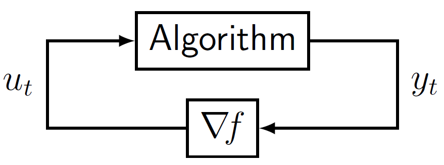
Optimization problems in engineering and applied mathematics are typically solved in an iterative fashion, by systematically adjusting the variables of interest until an adequate solution is found. The iterative algorithms that govern these systematic adjustments can be viewed as a control system (diagram shown right). The “Algorithm” block is a discrete-time dynamical system representing the algorithm, and the block $\nabla\!f$ is the gradient of the function we are optimizing. The difference between this setup and the spring-mass-damper system discussed above is that here, our task is to design one algorithm for use with a variety of different functions $f$. We would like an assurance that for all $f$ within the class of interest, the system is stable. specifically, we want $\lim_{t\to\infty} u(t) = 0$, $\lim_{t\to\infty} y(t) = y^\star$, because this means we have found a point at which the gradient is zero. Namely, $\nabla\! f(y_\star) = 0$, so $y_\star$ is a minimizer of $f$. Ensuring stability for all systems within a given class is called robust stability.

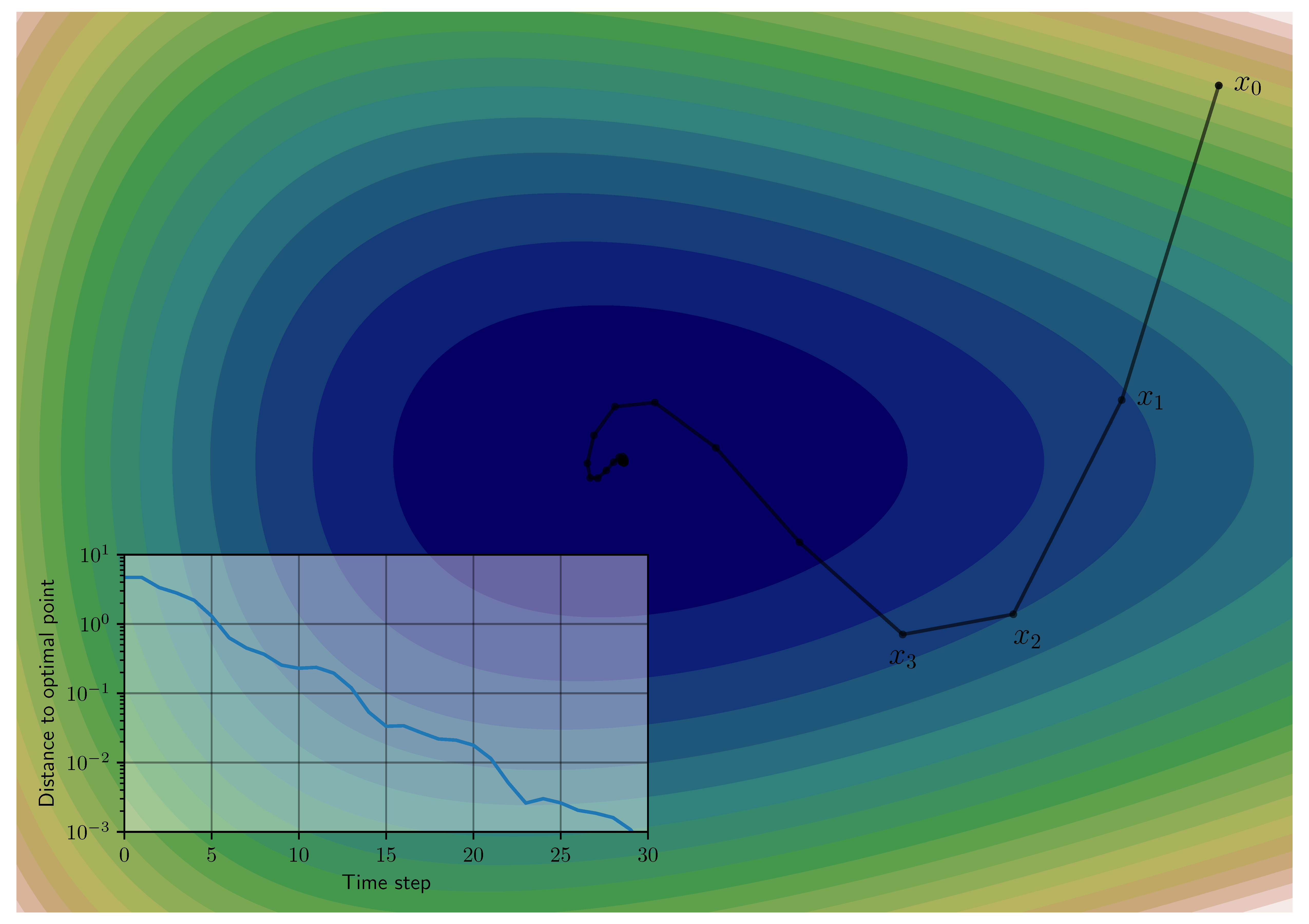
We can apply the dissipativity idea to the problem of robust stability by viewing the algorithm block as separate from the gradient $\nabla\!f$. Specifically, we characterize $\nabla\!f$ in terms of the supply rates it can provide. For example, suppose we know that $f$ is a convex function. Convex functions have monotone gradients, which means that $f$ must satisfy the inequality $(\nabla\! f(x_1)-\nabla\! f(x_2))^\mathsf{T}(x_1-x_2) \geq 0$. Put another way, any two inputs $y_1$ and $y_2$ (and corresponding outputs $u_1$ and $u_2$) for the block $\nabla\!f$ satisfy the inequality: \[ -(u_1-u_2)^\mathsf{T}(y_1-y_2) \leq 0 \]We can use the left-hand side of this inequality as a supply rate! It plays a role similar to the friction term in the spring-mass-damper system; it is guaranteed to always be negative and therefore serves to dissipate energy from the system. The difference here is that we are not dealing with a mechanical system, but rather an optimization algorithm, so the notion of “energy” is more abstract. This more abstract notion of energy (storage function) takes the rough form: \[ V(x) = (x_t-x_\star)^\mathsf{T} P (x_t-x_\star) + (f_t-f_\star) \]The first term is a positive definite quadratic function of the distance to the optimal point (a “kinetic energy” term). The second term is the distance to the optimal point in terms of function value (a “potential energy” term). This flexible representation allows us to characterize the behavior of algorithms that are not “descent methods”. For example, accelerated methods such as Nesterov’s method typically do not make uniform progress toward their goal. Some iterations will see the function value increase, even though the goal is to eventually minimize the function value! Much in the same way that neither position nor velocity are good measures of progress for the spring-mass-damper system. The right way to view progress is by using a combination of position and velocity. The image on the right illustrates how “distance to optimality” may not make uniform progress even though the algorithm converges.

In my paper, I explain how to use dissipativity theory to analyze several different types of optimization algorithms: gradient descent, accelerated methods (such as Heavy-ball and Nesterov), methods for constrained optimization such as projected gradient descent, and operator-splitting methods such as the Alternating Direction Method of Multipliers (ADMM). The main benefit of using dissipativity for algorithm analysis is that it provides a simple and intuitive way to understand algorithm performance. Moreover, dissipation inequalities can be found in a systematic and computationally-efficient manner, which makes the algorithm selection and tuning process amenable to automation.

My article explaining dissipativity theory for algorithm analysis appeared in the June 2022 issue of the IEEE Control Systems Magazine. A preprint version of the article is available for free here.