A polyhedron has six edges. Five of the edges have length $1$. What is the largest possible volume?
Here is my solution
[Show Solution]
A blog for mathematical riddles, puzzles, and elegant proofs

A polyhedron has six edges. Five of the edges have length $1$. What is the largest possible volume?
Here is my solution
[Show Solution]
The only polyhedron with six edges is a tetrahedron, which is a pyramid with a triangular base. Two of the faces will be equilateral triangles that share a common edge. This accounts for the five edges of length 1. The length of the sixth edge is determined by the angle between the faces, which we will call $\theta$. Here is an animation showing the different tetrahedra you get as you vary $\theta$:
In this diagram, $AB=BC=AC=AD=BD=1$ and $OD=OC=\frac{\sqrt{3}}{2}$.
The volume is equal to
\begin{align}
V&=\frac{1}{3}(\text{Area of base})\cdot(\text{altitude}) \\
&= \frac{1}{3}(\text{Area ABC})\cdot(DG) \\
&= \frac{1}{3}\left( \frac{1}{2} (AB)(OC) \right) \cdot \left( (OD) \sin\theta \right) \\
&= \frac{1}{3} \cdot \frac{1}{2}\cdot 1 \cdot \frac{\sqrt{3}}{2} \cdot \frac{\sqrt{3}}{2} \cdot \sin\theta \\
&= \frac{1}{8}\cdot\sin\theta
\end{align}Therefore, the maximum volume is $\frac{1}{8}$ and it occurs when $\theta=90^\circ$. This is intuitive because the area of the base is fixed, so the largest volume occurs when the altitude is as large as possible.

You will be asked four seemingly arbitrary true-or-false questions by the Sphinx on a topic about which you know absolutely nothing. Before the first question is asked, you have exactly $1. For each question, you can bet any non-negative amount of money that you will answer correctly. That is, you can bet any real number (including fractions of pennies) between zero and the current amount of money you have. After each of your answers, the Sphinx reveals the correct answer. If you are right, you gain the amount of money you bet; if you are wrong, you lose the money you bet.
However, there’s a catch. (Isn’t there always, with the Sphinx?) The answer will never be the same for three questions in a row.
With this information in hand, what is the maximum amount of money you can be sure that you’ll win, no matter what the answers wind up being?
Extra credit: This riddle can be generalized so that the Sphinx asks N questions, such that the answer is never the same for Q questions in a row. What are your maximum guaranteed winnings in terms of N and Q?
If you’re just looking for the answer, here it is:
[Show Solution]
Suppose there are $N$ total questions, and the Sphinx never gives the same answer $Q$ times in a row.
Define $F^{Q}_{n}$ to be the $n^\text{th}$ $Q$-generalized Fibonacci number. Specifically:
\begin{align}
F^Q_{n} &= 0 & \text{for }n \leq 0 \\
F^Q_1 &= 1 \\
F^Q_n &= F^Q_{n-1} + F^Q_{n-2} + \cdots + F^Q_{n-Q} & \text{for }n \geq 2
\end{align}These are also called Fibonacci $Q$-step numbers. Here are some examples (borrowed from here)
| $Q$ | OEIS | Name | sequence $F^{Q}_{n}$ starting at $n=0$ |
| 1 | degenerate | 0, 1, 1, 1, 1, 1, 1, 1, 1, 1, 1, … | |
| 2 | A000045 | Fibonacci | 0, 1, 1, 2, 3, 5, 8, 13, 21, 34, 55, … |
| 3 | A000073 | tribonacci | 0, 1, 1, 2, 4, 7, 13, 24, 44, 81, … |
| 4 | A000078 | tetranacci | 0, 1, 1, 2, 4, 8, 15, 29, 56, 108, … |
| 5 | A001591 | pentanacci | 0, 1, 1, 2, 4, 8, 16, 31, 61, 120, … |
| 6 | A001592 | hexanacci | 0, 1, 1, 2, 4, 8, 16, 32, 63, 125, … |
| 7 | A066178 | heptanacci | 0, 1, 1, 2, 4, 8, 16, 32, 64, 127, … |
The maximum amount of money we can expect to have after $N$ questions assuming optimal play is given by the formula:
$\displaystyle
\text{Maximum guaranteed winnings} = \frac{2^{N-1}}{F^{Q-1}_{N+1}}
$
Here is the optimal strategy that achieves this gain:
Note that as $q$ increases (the Sphinx is getting closer to being forced to answer predictably), the wagers get larger. When $q=Q-1$, the wager fraction simplifies to $1$, i.e. we should wager everything because we know we will win. When $n+q \lt Q$, there aren’t enough questions remaining to force the Sphinx to answer predictably, so we can expect to always lose and we should wager nothing.
Here is a plot showing the maximum guaranteed winnings as a function of $N$ and $Q$ if we start with \$1, which is given by the formula $\frac{2^{N-1}}{F^{Q-1}_{N+1}}$.

When $Q=2$, the Sphinx must alternate answers, so we can double our money every turn! This explains why the plot grows by a factor of 2 when $Q=2$ (the vertical axis is on a logarithmic scale). The plot is also flat for $N \leq Q-1$. This corresponds to the case where we have insufficient questions to force the Sphinx to answer predictably, so our best bet is to wager nothing and cut our losses.
In the detailed write-up, I explain how all of these formulas were derived, and I also go into detail on the asymptotic growth rate we can expect for different $Q$.
Here is a more detailed write-up of the solution:
[Show Solution]
We will solve the most general version of the problem, with $N$ questions and no $Q$ answers in a row are ever the same. This is a sequential decision-making problem, where at each turn of the game, we make a move (pick an answer and pick a wager), and then the Sphinx makes a move (picking the correct answer). We are looking to maximize our guaranteed winnings, which means we should assume the Sphinx is doing her best to minimize our winnings, while we are doing our best to maximize our winnings.
We will approach this problem using recursion, by expressing any given state of the game in terms of simpler states of the game. To do this, we must think about what constitutes a state of the game; what is the complete set of information that should be used to determine our next actions? Based on the rules of the game, the key pieces of information are:
Importantly, the current amount of money we have is irrelevant, because we will always wager some proportion of our current holdings. Likewise, the amount we win in the end will also be proportional to our current holdings. For example, any strategy that guarantees we will have \$1.50 at the end if we currently have \$1 can be used to guarantee us \$3 if we currently have \$2, or \$15 if we currently have \$10.
With this knowledge in mind, define $V_{q,n}^Q$ to be the amount we will have at the end if we start with \$1 and both players (us and the Sphinx) play perfectly, the current streak is at $q$ with a limit of $Q$, and we have $n$ turns remaining. Ultimately, our goal is to find $V_{0,N}^Q$, but we’ll find all possible values in the process of solving the problem. We’ll use a dynamic programming approach, starting from simple cases (small $n$) and working our way back to the general $n=N$ case. The function $V$ we defined is typically called the value function.
Let’s call $u$ the amount we wager, with $0\leq u \leq 1$. We can consider several base (or special) cases, for which the answer is immediately apparent. Here they are:
Case $n=0$. If there are no questions left to answer, the game is over and we take home the money we currently have. So we can write:
\[
V_{q,0}^Q = 1
\qquad\text{for all }q,Q.
\]
Case $n + q \lt Q$. If there aren’t enough questions remaining for the Sphinx to reset their streak quota, then the Sphinx can make us lose our remaining turns and they suffer no consequences. If we ever find ourselves in this situation, we should cut our losses and wager $u=0$. Therefore,
\[
V_{q,n}^Q = 1\qquad\text{if }q+n\lt Q\quad\text{with wager }u=0
\]
Case $q=Q-1$. This is the situation where the Sphinx’s hand is forced. They have already answered the same way $Q-1$ turns in a row, so they are forced to answer differently on their next turn, so we can bet everything we’ve got and we’re assured to win and double our money! Therefore, we should answer whatever the opposite to the current streak (i.e., if the correct answer was True $Q-1$ times in a row, we should answer the next question False) and we will win:
\[
V_{Q-1,n}^Q = 2 V_{1,n-1}^Q\qquad\text{and we should wager }u=1.
\]
Case $q=0$. This case is also interesting because it only happens at the start of the game. Once the game in underway, we have $q \geq 1$. So let’s see what happens on that first move. After our move, $n$ is reduced by one, and we either have $1+u$ or $1-u$, depending on whether we answered correctly or incorrectly.
\[
V_{0,n}^Q = \begin{cases}
(1+u)V_{1,n-1}^Q & \text{if we are correct} \\
(1-u)V_{1,n-1}^Q & \text{if we are incorrect}
\end{cases}
\]Keep in mind the Sphinx is out to ruin us, so for all intents and purposes, the Sphinx decides whether we are correct or not. No matter what happens, the Sphinx will accrue a streak of 1 so $q=1$. There is no trade-off here; the Sphinx can make us lose and it doesn’t cost her anything! We will lose any amount we bet, so the only safe move in this case is to bet nothing, and essentially skip our first turn. So we have:
\[
V_{0,n}^Q = V_{1,n-1}^Q
\qquad\text{and we should wager }u=0.
\]
In the general case, with a current streak of $1 \leq q \leq Q-2$ and $n$ questions left to answer, we can answer the same as the current streak, or answer differently. We can also be right or wrong. So there are four possibilities. The possibilities are:
\[
V_{q,n}^Q = \begin{cases}
\text{Answer same:} & \begin{cases}
(1+u)V^Q_{q+1,n-1} & \text{if correct} \\
(1-u)V^Q_{1,n-1} & \text{if incorrect}
\end{cases}\\
\text{Answer different:} & \begin{cases}
(1+u)V^Q_{1,n-1} & \text{if correct} \\
(1-u)V^Q_{q+1,n-1} & \text{if incorrect}
\end{cases}
\end{cases}
\]The Sphinx will always pick the option that causes us to lose as much as possible, so we can simplify this to:
\[
V_{q,n}^Q = \begin{cases}
\min\left\{ (1+u)V^Q_{q+1,n-1}, (1-u)V^Q_{1,n-1} \right\}
& \text{if we answer same}\\
\min\left\{ (1+u)V^Q_{1,n-1}, (1-u)V^Q_{q+1,n-1} \right\}
& \text{if we answer different}
\end{cases}
\]We can simplify further, by noting that $V^Q_{q,n}$ is an increasing function of $q$. In other words, the longer the current streak, the more we can expect to win, because we are closer to forcing an answer out of the Sphinx. These properties imply that $(1+u)V^Q_{q+1,n-1} \geq (1-u)V^Q_{1,n-1}$. So if we “answer same”, the Sphinx will always have us lose. Naturally, if we give the Sphinx an opportunity to take some of our money and reset its streak counter, of course she will take it! This drives us to the striking conclusion:
Always answer the opposite of the previous correct answer.
This simplifies things greatly, but we still don’t know how much to wager. We should wager an amount $u$ that maximizes our winnings assuming the Sphinx plays perfectly. Therefore:
\[
V_{q,n}^Q = \max_{0 \leq u \leq 1}
\min\left\{ (1+u)V^Q_{1,n-1}, (1-u)V^Q_{q+1,n-1} \right\}
\]In other words, we are presenting the Sphinx with a trade-off: she can choose to have us lose our wager, but this will bring her closer to filling her streak quota and forcing her hand. Or, she can reset her streak quota, but at the cost of having us win our wager.
Putting everything together, here are the dynamic programming recursions for our value function.
\begin{align}
V_{0,n}^Q &= V_{1,n-1}^Q\qquad\text{if }n\geq 1\quad\text{with wager }u=0\\
V_{q,0}^Q &= 1\qquad \text{for all }q\\
V_{q,n}^Q &= 1\qquad\text{if }q+n\lt Q\quad\text{with wager }u=0 \\
V_{Q-1,n}^Q &= 2V_{1,n-1}^Q\qquad\text{if }n\geq 1\quad\text{with wager }u=1 \\
V_{q,n}^Q &= \max_{0 \leq u \leq 1}
\min\left\{ (1+u)V^Q_{1,n-1}, (1-u)V^Q_{q+1,n-1} \right\},\\
&\quad \text{for }\quad 1\leq q \leq Q-2\text{ and }n\geq \max\{Q-q,1\}
\end{align}
The min/max optimization is now straightforward to solve. All functions involved are linear in $u$, so the optimum will occur either at a boundary ($u=0$ or $u=1$), or it will occur at the intersection of both functions. We already took care of all boundary cases, so we are now dealing with the latter case. Therefore, the optimal wager satisfies $(1+u)V^Q_{1,n-1}=(1-u)V^Q_{q+1,n-1}$, which leads to:
\[
u_\text{opt} = \frac{V^Q_{q+1,n-1}-V^Q_{1,n-1}}{V^Q_{q+1,n-1}+V^Q_{1,n-1}}
\quad\text{and}\quad
V^Q_{q,n} = \frac{2V^Q_{q+1,n-1}V^Q_{1,n-1}}{V^Q_{q+1,n-1}+V^Q_{1,n-1}}
\]Our simplified recursion is therefore:
\begin{align}
V_{0,n}^Q &= V_{1,n-1}^Q\qquad\text{if }n\geq 1\quad\text{with wager }u=0\\
V_{q,0}^Q &= 1\qquad \text{for all }q\\
V_{q,n}^Q &= 1\qquad\text{if }q+n\lt Q\quad\text{with wager }u=0 \\
V_{Q-1,n}^Q &= 2V_{1,n-1}^Q\qquad\text{if }n\geq 1\quad\text{with wager }u=1 \\
V_{q,n}^Q &= \frac{2V^Q_{q+1,n-1}V^Q_{1,n-1}}{V^Q_{q+1,n-1}+V^Q_{1,n-1}}
\quad\text{with wager }u = \frac{V^Q_{q+1,n-1}-V^Q_{1,n-1}}{V^Q_{q+1,n-1}+V^Q_{1,n-1}}\\
&\qquad\text{for }\quad 1\leq q \leq Q-2\text{ and }n\geq \max\{Q-q,1\}
\end{align}This still looks complicated, but we can make one last simplification. Notice that our only messy expression is the general recursion, which looks like $v = \frac{2ab}{a+b}$. We can rewrite this as: $\frac{1}{v} = \frac{1}{2}\left( \frac{1}{a} + \frac{1}{b} \right)$, which looks much nicer. To this effect, let’s make this change of variables:
\[
W^Q_{q,n} := \frac{2^n}{V^Q_{q,n}} \qquad\text{for all }Q,q,n.
\]With this change of variables, the recursion becomes linear!
\begin{align}
W_{0,n}^Q &= 2 W_{1,n-1}^Q\qquad\text{if }n\geq 1\quad\text{with wager }u=0\\
W_{q,0}^Q &= 1\qquad \text{for all }q\\
W_{q,n}^Q &= 2^n\qquad\text{if }q+n\lt Q\quad\text{with wager }u=0 \\
W_{Q-1,n}^Q &= W_{1,n-1}^Q\qquad\text{if }n\geq 1\quad\text{with wager }u=1 \\
W_{q,n}^Q &= W^Q_{1,n-1} + W^Q_{q+1,n-1}
\quad\text{with wager }u = \frac{W^Q_{1,n-1}-W^Q_{q+1,n-1}}{W^Q_{1,n-1}+W^Q_{q+1,n-1}}\\
&\qquad\text{for }\quad 1\leq q \leq Q-2\text{ and }n\geq \max\{Q-q,1\}
\end{align}
Let’s start with the case $q=1$, so we’ll solve for $W^Q_{1,n}$. Applying the last three recursions, we get:
\begin{align}
W^Q_{1,n} &= 2^n \qquad\text{for }0 \leq n \leq Q-2 \\
W^Q_{1,n} &= W^Q_{1,n-1} + W^Q_{1,n-2} + \cdots + W^Q_{1,n-(Q-1)}\qquad\text{for }n \geq Q-1
\end{align}This further simplifies to the compact form:
\begin{align}
W^Q_{1,-k} &= 0 \qquad \text{for all }k\geq 2\\
W^Q_{1,-1} &= 1 \\
W^Q_{1,n} &= W^Q_{1,n-1} + W^Q_{1,n-2} + \cdots + W^Q_{1,n-(Q-1)}\qquad\text{for }n \geq 0.
\end{align}The sequence of $W^Q_{1,n}$ are none other than generalized Fibonacci numbers! I guess we could call them $Q$bonacci numbers? When $Q=3$, we recover the standard Fibonacci numbers (A000045):
\[
\{1,1,2,3,5,8,13,21,\dots\}
\]but shifted by 2 (we are indexing starting from -1 here, but typically Fibonacci numbers are defined where the first “1” occurs at index 1). When $Q=4$, we obtain the so-called Tribonacci numbers (A000073):
\[
\{1,1,2,4,7,13,24,44,\dots\}
\]again shifted by 2. Let’s rename the sequence so it coincides with the standard generalized Fibonacci number naming convention.
\[
F^Q_n := W^{Q+1}_{1,n-2}
\]
We can derive the rest of the $W^Q_{q,n}$ by again using the recursion, and this allows us to write all $W^Q_{q,n}$ in terms of the $Q$bonacci numbers.
\begin{align}
W^Q_{q,n}
&= W^Q_{1,n-1} + W^Q_{1,n-2} + \cdots + W^Q_{1,n-(Q-q)} \\
&= F^{Q-1}_{n+1} + F^{Q-1}_{n} + \cdots + F^{Q-1}_{n-(Q-q)+2}
\end{align}Converting back to the value function notation, we can write a formula for $V^Q_{q,n}$ and the optimal wager $U^Q_{q,n}$ in terms of the $Q$bonacci numbers:
\[
\begin{aligned}
V^Q_{0,n} &= V^Q_{1,n-1} = \frac{2^{n-1}}{W^Q_{1,n-1}} = \frac{2^{n-1}}{F^{Q-1}_{n+1}} \\
U^Q_{0,n} &= 0 \\
V^Q_{q,n} &= \frac{2^n}{W^Q_{q,n}} = \frac{2^n}{F^{Q-1}_{n+1} + F^{Q-1}_{n} + \cdots + F^{Q-1}_{n-(Q-q)+2}}\qquad\text{for }1\leq q \leq Q-1\\
U^Q_{q,n} &= \frac{2F^{Q-1}_{n+1}}{F^{Q-1}_{n+1} + F^{Q-1}_{n} + \cdots + F^{Q-1}_{n-(Q-q)+2}}-1
\end{aligned}
\]
Therefore, the solution to the original question, how much money can we be guaranteed to win if we wager optimally, is given by the formula
$\displaystyle
V^Q_{0,N} = \frac{2^{N-1}}{F^{Q-1}_{N+1}}
$
We might also be interested in the limit $N\to\infty$. In other words, what will our asymptotic growth rate look like if $N$ is much larger than $Q$? The generalized Fibonacci numbers have an asymptotically exponential growth, because they are solutions of a linear recurrence. This leads to Binet’s formula for the $n^\text{th}$ Fibonacci number:
\[
F^2_n = \frac{1}{\sqrt{5}}\left( \left(\frac{1+\sqrt{5}}{2}\right)^n – \left(\frac{1-\sqrt{5}}{2}\right)^n \right)
\]In spite of the $\sqrt{5}$ terms, this formula always produces integers! The asymptotic growth of $F^2_n$ is dictated by the term with the largest magnitude. In this case, $F^2_n \sim O\left( \varphi^n \right)$, where $\varphi = \frac{1+\sqrt{5}}{2}$ is the golden ratio. The Binet formula can also be generalized for $Q \gt 2$, and so can the asymptotic rate. The following paper by Dresden and Du does just this. I will summarize the key result.
\[
F^Q_n = O(\alpha^n)
\]Where $\alpha$ is the positive real root (there is only one) of the equation
\[
\alpha^Q = \alpha^{Q-1} + \alpha^{Q-2} + \cdots + \alpha + 1
\]In general, this polynomial will have one root that is positive and less than 2, and the other roots will be negative or complex and will have magnitude less than 1. In the paper, the authors prove that $\alpha$ increases as we increase $Q$, and $2-\frac{1}{Q} \lt \alpha \lt 2$. The growth rate of our earnings is given by $\frac{2}{\alpha}$. Here is what we obtain for different values of $Q$:
| Q | Growth rate $\frac{2}{\alpha}$ |
| 2 | 2 |
| 3 | 1.236068 |
| 4 | 1.087378 |
| 5 | 1.0375801 |
| 6 | 1.0173208 |
| 7 | 1.00827652 |
| 8 | 1.00403411 |
| 9 | 1.00198836 |
| 10 | 1.000986237 |
There is no known closed-form expression for $\alpha$ when $Q \geq 5$ as quintics (polynomials of degree $5$) are not solvable using standard functions like square roots, but it is easy enough to approximate. One way to do this is to notice that the polynomial that defines $\alpha$ is precisely the characteristic polynomial of the $Q\times Q$ matrix:
\[
A = \begin{bmatrix}
0 & 1 & 0 & \cdots & 0 \\
0 & 0 & 1 & \ddots & 0 \\
\vdots & \vdots & \ddots & \ddots & \vdots \\
0 & 0 & \cdots & 0 & 1 \\
1 & 1 & \cdots & 1 & 1
\end{bmatrix} \in \mathbb{R}^{Q\times Q}
\]Therefore $\alpha = \rho(A)$ is spectral radius of the matrix $A$. This can be found efficiently using something like the Power Iteration, particularly because this top eigenvalue is so well-separated from the other eigenvalues, which have magnitude less than 1.
You have a sheet of crust laid out in front of you. After baking, your pie crust will be a cylinder of uniform thickness (or rather, thinness) with delicious filling inside.
To maximize the volume of your pie, what fraction of your crust should you use to make the circular base (i.e., the bottom) of the pie?
Here is my solution:
[Show Solution]
Since we have a fixed amount of crust that we will shape into a cylinder, the problem is one of maximizing the volume for a fixed area. This is known as the isovolume problem (which is a misnomer; it should really be called the isoarea problem).
Let’s suppose the crust has an area of $A$. Given this area, we would like to maximize the volume of the cylinder. Let’s suppose the radius of the base is $r$ and the height is $h$. Then the formulas are:
\[
A = 2\pi r^2 + 2\pi r h \qquad\text{and}\qquad V = \pi r^2 h.
\]Since the area $A$ is fixed, we are not free to choose $r$ and $h$ independently. Once $r$ is chosen, $h$ is uniquely determined by the equation for $A$. Solving for $h$ in terms of $A$ from the area equation, we obtain:
\[
h = \frac{A-2\pi r^2}{2\pi r}
\]Substituting this value of $h$ into the equation for $V$, we obtain:
\[
V= \frac{1}{2} r (A-2\pi r^2)
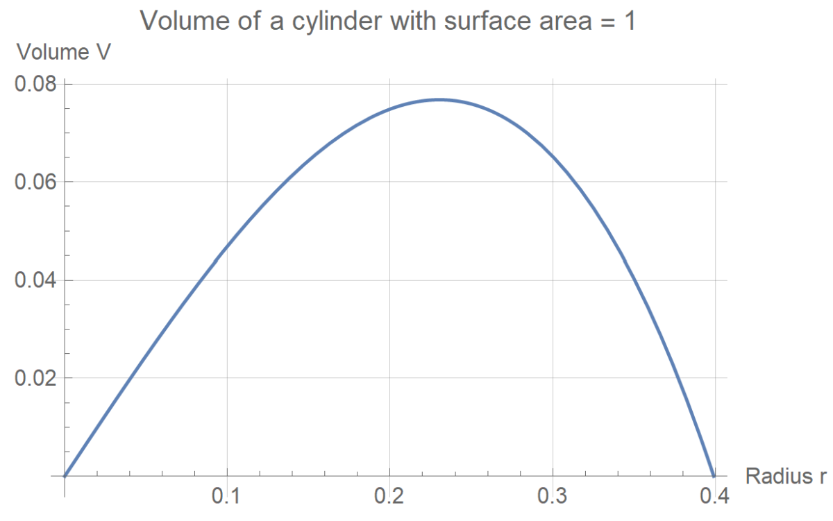
\]Here is a plot of what this function $V(r)$ looks like for a value of $A=1$:

We can maximize $V$ by looking for an $r$ such that $\frac{\mathrm{d}V}{\mathrm{d}r}=0$ and $\frac{\mathrm{d}^2V}{\mathrm{d}r^2}\lt 0$. In other words, at the optimal choice of $r$, the tangent to the curve $V(r)$ is flat and the curvature is negative (curves downward). This leads to the equations:
\[
\frac{1}{2}(A-6\pi r ^2) = 0 \qquad\text{and}\qquad -6\pi r \lt 0
\]Since $r\geq 0$ (radius can’t be negative), the second equation is always satisfied, and the first equation implies that $r=\sqrt{\frac{A}{6\pi}}$. If $A=1$ as in the plot above, this leads to $r=0.23033$, which looks about right! With the optimal choice of $r$, the corresponding choice of $h$ becomes $h=\sqrt{\frac{2A}{3\pi}}$ and the corresponding optimal volume is $V=\frac{A^{3/2}}{3\sqrt{6\pi}}$. Interestingly, we can observe that with these choices,
\[
2r = 2\sqrt{\frac{A}{6\pi}} = \sqrt{\frac{4A}{6\pi}} = \sqrt{\frac{2A}{3\pi}} = h
\]So in order to maximize the area, the diameter should be equal to the height! In other words, when viewed from the side, our pie should have a square shape; we’ll be making more of a cake rather than a pie.
The fraction of crust used for the base of the optimal pie is:
\[
\frac{\pi r^2}{A} = \frac{\pi \left(\frac{A}{6\pi}\right)}{A} = \frac{1}{6}.
\]
$\displaystyle
\begin{aligned}
&\text{So we should use $\tfrac{1}{6}$ of the crust for the base, $\tfrac{1}{6}$ for the top,}\\
&\text{and the remaining $\tfrac{2}{3}$ for the sides.}
\end{aligned}$
One way to explain the shape of this tall pie is to think back to the isovolume problem discussed earlier. The solution to the isovolume problem is a sphere. So in order to be as efficient as possible, the pie’s shape should be as close to a sphere as possible, hence the tall shape. For a sphere, $A=4\pi r^2$ and $V=\frac{4}{3}\pi r^3$, so by eliminating $r$, we obtain $V=\frac{A^{3/2}}{6\sqrt{\pi}}$.
If we take the ratio of the volume of the sphere and the volume of the optimized cylinder, we obtain:
\[
\frac{V_\text{cylinder}}{V_\text{sphere}} = \frac{ \frac{A^{3/2}}{3\sqrt{6\pi}} }{ \frac{A^{3/2}}{6\sqrt{\pi}} } = \sqrt{\frac{2}{3}} \approx 0.8165
\]So the optimized cylindrical pie will have a volume which is about 82% of the largest possible volume.
If the top and bottom areas of the pie have different radii, then the shape is no longer a cylinder, but rather a frustom of a cone. The formulas are now a bit more complicated, because they depend on two radii ($r$ and $R$) and the height $h$:
\begin{align}
A &= \pi (r+R) \sqrt{h^2+(R-r)^2}+\pi \left(r^2+R^2\right)\\
V &= \frac{1}{3} \pi h \left(r^2+r R+R^2\right)
\end{align}Using a similar procedure as before (solving for $h$ in the area equation and substituting this into the volume equation), we obtain the following volume formula that depends only on the radii of the top and bottom
\[
V = \frac{\left(r^2+r R+R^2\right) \sqrt{\left(A-2 \pi r^2\right) \left(A-2 \pi R^2\right)}}{3 (r+R)}
\]A necessary condition for optimality is that both partial derivatives are zero, namely $\frac{\partial V}{\partial r} = \frac{\partial V}{\partial R} = 0$. This leads to the equations:
\begin{align}
\frac{\partial V}{\partial r} &= -\frac{r \left(A-2 \pi R^2\right) \left(2 \pi \left(4 r^2 R+2 r^3+2 r R^2+R^3\right)-A (r+2 R)\right)}{3 (r+R)^2 \sqrt{\left(A-2 \pi r^2\right) \left(A-2 \pi R^2\right)}} \\
\frac{\partial V}{\partial R} &= -\frac{R \left(A-2 \pi r^2\right) \left(2 \pi \left(2 r^2 R+r^3+4 r R^2+2 R^3\right)-A (2 r+R)\right)}{3 (r+R)^2 \sqrt{\left(A-2 \pi r^2\right) \left(A-2 \pi R^2\right)}}
\end{align}Much messier than the ordinary cylinder case… But we can simplify this. It must be true that $A\gt 2\pi R^2$ and $A\gt 2\pi r ^2$, since the area of the smaller circle plus the area of the sides must be at least the area of the larger circle (they are only equal when the pie is flat). So if $\frac{\partial V}{\partial r} = \frac{\partial V}{\partial R} = 0$, we can cancel a bunch of terms and we are left with:
\begin{align}
2 \pi \left(4 r^2 R+2 r^3+2 r R^2+R^3\right)-A (r+2 R) &= 0& &(1) \\
2 \pi \left(2 r^2 R+r^3+4 r R^2+2 R^3\right)-A (2 r+R) &= 0& &(2)
\end{align}This still looks rather messy to solve, but we can make a clever observation. If we subtract one equation from the other $(2)-(1)$ and factor, we obtain:
\[
(R-r) \left(A+2 \pi r^2+6 \pi r R+2 \pi R^2\right)=0
\]The right factor consists of a sum of positive terms, and therefore must be positive. So we conclude that $R=r$. Put another way, the only way we’ll have an optimized volume is if the top and bottom circles are of equal size. This reduces our more complicated case to the simpler case we already solved above.

You want to build a polygonal enclosure consisting of posts connected by walls. Each post weighs $k$ kg. The walls weigh $1$ kg per meter. You are allowed a maximum budget of $1$ kg for the posts and walls.
What’s the greatest value of $k$ for which you should use four posts rather than three?
Extra credit: For which values of $k$ should you use five posts, six posts, seven posts, and so on?
Here is my solution:
[Show Solution]
For a fixed perimeter, the maximum-area polygon with $n$ sides is a regular polygon. Since we are interested in maximizing area, we should therefore always use regular polygons as our shape, and we should always use our entire mass budget of $1$ kg.
Let’s assume the weight of the posts $k$ is given and fixed. If the perimeter is $p$ and the number of sides is $n$, the formula for the area of a regular $n$-gon is as follows (explanation here).
\[
A = \frac{p^2}{4n \tan\frac{\pi}{n}}
\]Our total budget constraint is that $p + kn \leq 1$. Since our goal is to maximize area we should always use our entire budget. So $p = 1-kn$. This means that $n \leq \frac{1}{k}$ in order to ensure we respect the weight budget. So for a fixed $k$, the maximum area of an $n$-gon enclosure is given by the formula
$\displaystyle
A = \frac{(1-kn)^2}{4n\tan\frac{\pi}{n}}\qquad\text{for: }2\leq n \leq \frac{1}{k}
$
Let’s talk about limiting cases for a moment.
So for each $k$, we should choose the $n \in \{2,3,4,\dots,\lfloor \tfrac{1}{k}\rfloor\}$ that maximizes $A$. Here is a plot showing plots of $A$ for each $n$ and $k$. When $k$ is large (posts weigh a lot), we try to use as few of them as possible. So at first, the triangle ($n=3$) is best. As we decrease $k$, it eventually becomes more efficient to use a square ($n=4$), and so on. As $k$ goes to zero, we obtain the solution with $n\to\infty$, which is the circular enclosure discussed above.

To find out where the transition occurs between $n$ and $n+1$, we should look for the value of $k$ at which the areas match (indicated by the black dots on the plot). So we want to find $k$ such that:
\[
\frac{(1-kn)^2}{4n\tan\frac{\pi}{n}} = \frac{(1-k(n+1))^2}{4(n+1)\tan \frac{\pi}{n+1}}
\]Solving this equation for $k$, we obtain:
$\displaystyle
k_n = \frac{ \sqrt{n \tan \frac{\pi}{n}}-\sqrt{(n+1) \tan \frac{\pi}{n+1}} }{ (n+1)\sqrt{n \tan \frac{\pi}{n}}-n\sqrt{(n+1) \tan \frac{\pi}{n+1}} }
$
We can interpret this formula as follows: $k_n$ is the smallest value of $k$ for which we should use $n$ posts in our enclosure. So if we make $k$ smaller, it becomes more efficient to use $(n+1)$ posts instead. Here are the first few numerical values of $k_n$:
| $n$ | $k_n$ | Range of $k$ for this $n$ |
|---|---|---|
| $2$ | $0.333333$ | $0.333333 \leq k$ |
| $3$ | $0.089642$ | $0.089642 \leq k \leq 0.333333$ |
| $4$ | $0.039573$ | $0.039573 \leq k \leq 0.089642$ |
| $5$ | $0.021016$ | $0.021016 \leq k \leq 0.039573$ |
| $6$ | $0.012511$ | $0.012511 \leq k \leq 0.021016$ |
| $7$ | $0.008056$ | $0.008056 \leq k \leq 0.012511$ |
| $8$ | $0.005494$ | $0.005494 \leq k \leq 0.008056$ |

Antisocial settlers are building houses on a prairie that’s a perfect circle with a radius of 1 mile. Each settler wants to live as far apart from his or her nearest neighbor as possible. To accomplish that, the settlers will overcome their antisocial behavior and work together so that the average distance between each settler and his or her nearest neighbor is as large as possible.
At first, there were slated to be seven settlers. Arranging that was easy enough: One will build his house in the center of the circle, while the other six will form a regular hexagon along its circumference. Every settler will be exactly 1 mile from his nearest neighbor, so the average distance is 1 mile.
However, at the last minute, one settler cancels his move to the prairie altogether (he’s really antisocial). That leaves six settlers. Does that mean the settlers can live further away from each other than they would have if there were seven settlers? Where will the six settlers ultimately build their houses, and what’s the maximum average distance between nearest neighbors?
Here is my solution:
[Show Solution]
I approached this problem from a modeling and optimization perspective. If there are $N$ settlers and we imagine the coordinates of the settlers are $(x_i,y_i)$ for $i=1,\dots,N$ and $d_i$ is the distance between the $i^\text{th}$ settler and its nearest neighbor, then we can model the problem as follows:
\[
\begin{aligned}\underset{x,y,d\,\in\,\mathbb{R}^N}{\text{maximize}} \quad & \frac{1}{N}\sum_{i=1}^N d_i \\
\text{such that} \quad & x_i^2 + y_i^2 \le 1 &&\text{for }i=1,\dots,N\\
& (x_i-x_j)^2 + (y_i-y_j)^2 \ge d_i^2 &&\text{for }i,j=1,\dots,N\text{ and }j\ne i
\end{aligned}
\]The objective is to minimize the average distance between each settler and its nearest neighbor (the average of the $d_i$). The first constraint says that each settler must be within the circle (a distance of at most $1$ from the origin). The second constraint says that the $i^\text{th}$ settler is a distance at least $d_i$ from each of the other settlers.
The game is then to find $(x_i,y_i,d_i)$ that satisfy these constraints and maximize the objective. Broadly speaking, this is an example of a mathematical optimization problem. Unfortunately, the problem as stated is nonconvex problem because of the form of the second constraint. This means that the problem may have local maximizers that are not globally optimal. There are two ways forward:
First, we could use local search: start with randomly placed settlers, wiggle their positions in ways such that the objective continues to increase, and then stop once we can no longer improve the objective. Examples of such approaches include hill-climbing and interior-point methods. In general, such approaches only find local maxima, so we should try many random starting positions to ensure we find the best possible answer.
Second, we could use global search: these are methods that attempt to find a globally optimal solution by considering many configurations simultaneously and adding random perturbations that can “kick” a solution out of a local maximum. Examples include simulated annealing and particle swarms. These approaches tend to be much slower than local search, but they have a much better chance of finding a global optimum.
Ultimately, I used local search with several random initializations. Here is how the maximum average distance scales with the number of settlements.

The bar plot also shows how well we would do if we distributed the settlements evenly on the circumference (“all on the border”) and if we put one in the middle and the rest evenly distributed on the circumference (“one in the center”). We can also examine what the settlement distributions actually look like. Here they are:

The case $N=6$ is particularly interesting because it has a settlement that is almost in the center, but not quite. Indeed, the average minimum distance to neighbors for this case is $1.002292$, so we benefit ever so slightly by placing one settlement off-center.
We can solve for the $N=6$ case analytically as well, but the solution isn’t pretty (fair warning!) It turns out the settlements are distributed throughout the circle in the following way:

Here, $x$ is the distance between the origin and the point $A$. The other distances satisfy $z \lt y \lt x+1$, and the average distance to the nearest neighbor is therefore $\tfrac{1}{6}(1+x+2y+3z)$. Note that once we set $x$, this uniquely determines the positions of all the other points. After some messy trigonometry, we obtain the following equations relating $x$, $y$, $z$ and two auxiliary variables $p$ and $q$:
\begin{align}
y^2&=1+x-x^2-x^3\\
z^2&=1-x^2+2x\left(pq-\sqrt{1-p^2}\sqrt{1-q^2}\right) \\
p&= \tfrac{1}{2}(1-2x-x^2)\\
q&= \tfrac{1}{2}(1-x+x^2+x^3)
\end{align}We can eliminate $\{y,z,p,q\}$ and solve for the average distance $\bar d = \frac{1+x+2y+3z}{6}$ as a function of $x$ alone:
\[
\bar d = \frac{x+1}{12} \left(2+4 \sqrt{1-x}+3 \sqrt{2}\sqrt{1-x} \sqrt{\left(x^3+2 x^2-x+2\right)-x \sqrt{x+3} \sqrt{x^3+x^2-x+3}} \right)
\]We can then plot this function of $x$, and we get the following curve:

Interestingly, this function reaches its maximum just a bit after $x=0$. Zooming in, we can see more clearly:

The maximum occurs at about $x=0.0555108$ and the maximum value is $1.00229$, just as we found before. If we try to solve for this analytically by taking the derivative of this function, setting it equal to zero, and eliminating rationals, we obtain the following result… That the optimal $x$ a root of the following $30^\text{th}$ order polynomial:
\begin{align}
x^{30}&+\tfrac{152}{9} x^{29}+\tfrac{9259}{81} x^{28}+\tfrac{6851}{18} x^{27}+\tfrac{383363 }{648}x^{26}+\tfrac{1999495} {5832}x^{25}\\
&+\tfrac{43478263}{52488} x^{24}+\tfrac{75726373}{23328} x^{23}+\tfrac{3282369305}{1679616} x^{22}-\tfrac{31642768891}{7558272} x^{21}\\
&+\tfrac{367775655235}{136048896} x^{20}+\tfrac{392027905801}{34012224} x^{19}-\tfrac{2016793647847}{136048896} x^{18}-\tfrac{1258157703385}{68024448} x^{17}\\
&+\tfrac{4545130566235}{136048896} x^{16}-\tfrac{22059424877}{17006112} x^{15}-\tfrac{8448216227365}{136048896} x^{14}+\tfrac{2878062707167}{68024448} x^{13}\\
&+\tfrac{7398046956073}{136048896} x^{12}-\tfrac{312655708903}{3779136} x^{11}+\tfrac{17266856539}{1679616} x^{10}+\tfrac{63670102441}{839808} x^9\\
&-\tfrac{29827845749}{559872} x^8-\tfrac{541401565}{23328} x^7+\tfrac{619158287}{23328} x^6+\tfrac{6168305}{2592} x^5\\
&-\tfrac{156285}{32} x^4-\tfrac{5153}{36} x^3+\tfrac{3923}{12} x^2+\tfrac{45}{2} x-\tfrac{35}{16}
\end{align}Yuck! Here is what you get if you plot this polynomial; as expected, there is a root at $x=0.0555108$.

As you may know, having one child, let alone many, is a lot of work. But Alice and Bob realized children require less of their parents’ time as they grow older. They figured out that the work involved in having a child equals one divided by the age of the child in years. (Yes, that means the work is infinite for a child right after they are born. That may be true.)
Anyhow, since having a new child is a lot of work, Alice and Bob don’t want to have another child until the total work required by all their other children is 1 or less. Suppose they have their first child at time T=0. When T=1, their only child is turns 1, so the work involved is 1, and so they have their second child. After roughly another 1.61 years, their children are roughly 1.61 and 2.61, the work required has dropped back down to 1, and so they have their third child. And so on.
(Feel free to ignore twins, deaths, the real-world inability to decide exactly when you have a child, and so on.)
Five questions: Does it make sense for Alice and Bob to have an infinite number of children? Does the time between kids increase as they have more and more kids? What can we say about when they have their Nth child — can we predict it with a formula? Does the size of their brood over time show asymptotic behavior? If so, what are its bounds?
Here is an explanation of my derivation:
[Show Solution]
Let’s call $t_k$ the time at which Alice and Bob have their $k^\text{th}$ child. The first child is born at time zero, so $t_1 = 0$. Since the work due to a child is one divided by their age, the work due to child $k$ at time $t$ is given by:
\[
\text{work at time }t = \begin{cases}
\frac{1}{t-t_k} & \text{if }t > t_k \\
0 & \text{otherwise}
\end{cases}
\]We also know that each new child is born once the total work due to all previous children equals $1$. Therefore, we have the following equations:
\begin{align}
t_2\text{ satsifies:} && \frac{1}{t_2-t_1} &= 1 \\
t_3\text{ satisfies:} && \frac{1}{t_3-t_2} + \frac{1}{t_3-t_1} &= 1 \\
t_4\text{ satisfies:} && \frac{1}{t_4-t_3} + \frac{1}{t_4-t_2} + \frac{1}{t_4-t_1} &= 1 \\
\cdots\qquad \\
t_k\text{ satisfies:} && \sum_{i=1}^{k-1} \frac{1}{t_k-t_i} &= 1
\end{align}and so on. We also know that $t_1 \lt t_2 \lt t_3 \lt \ldots$ since the children are born sequentially. The nice thing about these equation is that they can be solved sequentially. We know that $t_1=0$. Substituting this into the first equation yields $t_2=1$. Substituting these values into the second equation yields:
\[
\frac{1}{t_3-1}+\frac{1}{t_3} = 1
\]Rearranging yields $t_3^2-3t_3+1=0$. This equation has two solutions, but we take the one that satisfies $t_3 \gt t_2$, and we obtain $t_3=\tfrac{3+\sqrt{5}}{2} \approx 2.618$. We can continue in this fashion, solving each subsequent equation by substituting the previous values… but things get complicated in a hurry. The next equation becomes:
\[
t_4^3-\left(\tfrac{11+\sqrt{5}}{2}\right)t_4^2+\left(\tfrac{13+3\sqrt{5}}{2}\right)t_4-\left(\tfrac{3+\sqrt{5}}{2}\right)=0
\]Once again, we find that there is a unique solution that satisfies $t_4 \gt t_3$. This solution is approximately $t_4\approx 4.5993$. There doesn’t appear to be any automatic way to continue this process. Every time we try to compute the next $t_k$, we have to find the root of an even more complicated polynomial!
We’ll take a numerical approach, but let me first address one issue: how can we be sure that these ever-more-complicated polynomials always have a root that satisfies our constraints? For example, what if the polynomial for $t_4$ had no roots larger than $t_3$? What if it had many such roots? Thankfully, there is a simple way we can guarantee that there is always exactly one admissible root to each polynomial by leveraging the intermediate value theorem. Specifically, the function
\[
f_k(t) = \frac{1}{t-t_1} + \frac{1}{t-t_2} + \cdots + \frac{1}{t-t_{k-1}}
\]with $t \gt t_{k-1} \gt \ldots \gt t_1$ is a continuous and strictly decreasing function. Moreover, $\lim_{t\to {t_{k-1}}^+}f_k(t) = +\infty$ and $\lim_{t\to\infty} f_k(t) = 0$. Therefore, by the intermediate value theorem, there must be some point $t_k \in (t_{k-1},\infty)$ such that $f_k(t_k)=1$. The strict monoticity of $f_k$ ($f_k$ is strictly decreasing) implies that this $t_k$ must be unique.
The root may be unique, but how can we find it efficiently? Here, we can leverage a further property of $f_k$; namely convexity. The fact that $f_k$ is convex (and smooth) means that we can leverage some efficient methods from convex analysis that make use of derivative information. There are many ways to get the answer from here… What I ended up doing was to use the L-BFGS algorithm on the objective $(f_k(t)-1)^2$. My implementation in Julia using the Optim.jl package took about 40 seconds to evaluate birth dates of the first 1,000 children.
Note: there are many ways to formulate this as an optimization problem. One way is to note that solving $f_k(t)=1$ is equivalent to extremizing the antiderivative of $f_k(t)-1$. In other words, we could solve:
\[
t_k = \underset{t \gt t_{k-1}}{\text{arg min}} \left( t-\sum_{i=1}^{k-1}\log(t-t_i) \right)
= \underset{t \gt t_{k-1}}{\text{arg max}}\,\, e^{-t}\prod_{i=1}^{k-1}(t-t_i)
\]Incidentally, this last expression for $t_k$ makes it clear that there should be a unique $t_k$. When $t\gt t_{k-1}$, the product is a polynomial that is strictly increasing, and it’s multiplied by $e^{-t}$, which will drive it to zero eventually. There must therefore be a unique maximizer. I tried implementing both of these approaches and both turned out to be slower than directly minimizing $(f_k(t)-1)^2$.
If you’re just interested in the answers to the questions, here they are:
[Show Solution]

The first point on the left says that we wait $1$ year after child $1$ is born, we wait about $1.6$ years after child $2$ is born, and so on. Plotted on a log scale as above, we see the curve is almost a perfect straight line. Here is a formula we can use to approximate the number of years to wait:
$\displaystyle
\text{years to wait after child }k\text{ is born} \,\approx\, 1 + 2.19\cdot \log_{10} k
$
So yes, the time between children increases (without bound), but it does so slowly. By the time Alice and Bob have their 1,000th child, they will be waiting approximately 7.5 years between kids.
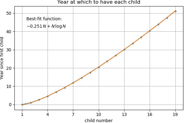
We can see here that the growth rate is slightly faster than linear. Since the time between children fit so well to a curve of the form $a+b\log x$, it makes sense to fit the birth dates themselves to the integral of this form. In an effort to fit the simplest possible curve, I did a bit of experimenting and found that the form $a x + x \log x$ does a really good job. I found the equation of best fit using linear regression and put the equation in the plot above. If we extend the time horizon, we get a similar result:

This is a pretty good fit; the plot actually depicts the true data with the fit overlaid on top. The fit is so good that you can’t even see the data underneath! So for large $N$, a good approximation is:
$\displaystyle
\text{year when child }N\text{ is born} \,\approx\,-0.315N + N\log N
$
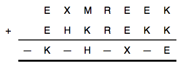
The goal is to decode two equations. In each of them, every different letter stands for a different digit. But there is a minor problem in both equations. In the first equation, letters accidentally were smudged and are now unreadable. (These are represented with dashes below.) But we know that all 10 digits, 0 through 9, appear in the equation.
What digits belong to what letters, and what are the dashes? In the second equation, one of the letters in the equation is wrong. But we don’t know which one. Which is it?
Here is my detailed solution:
[Show Solution]
This type of puzzle is called a cryptarithm, but this variant has the additional twist of smudges or errors that make the puzzle more challenging. Just like Sudoku, the puzzle involves filling numbers in a grid subject to several rules. Similarly, we can solve the problem by carefully and methodically deducing the solution using logic. In this post, I’m going to present a completely different approach; integer programming! By encoding the problem as an integer program, we can leverage powerful solvers to rapidly find the solution.
You might be thinking: if we’re asking a computer to solve the problem, then why not just have the computer check all possibilities? In this case, there are 10! = 3,628,800 different ways to assign the letters to the digits 0 through 9. This is certainly within the realm of possibility. I wrote code to do this and it took about 16 seconds to loop through all permutations. If we stop once we find a solution, we can expect this approach to take about 8 seconds. Not bad, but not particularly elegant either… I’ve included a link to all my code at the bottom of this post in case you’re interested in seeing how I went about coding it.
The secret code is:
\[
EXMREEK + EHKREKK = -K\!-\!H\!-\!X\!-\!E
\]The first thing to observe is that there are six distinct letters: $\{E,X,M,R,K,H\}$ and there are four smudges. Since each number 0 through 9 must appear exactly once, this tells us that the four smudges must correspond to different numbers. Therefore, we can add more variables and write the equation as:
\[
EXMREEK + EHKREKK = AKBHCXDE
\]
We will use ten binary numbers to encode each letter. For example, the letter $E$ is encoded using the list of binary numbers $\{E_0,E_1,\dots,E_9\}$ and represented as:
\[
E = E_1 + 2 E_2 + 3 E_3 + \cdots + 9 E_9
\]We then add the constraint:
\[
E_0 + E_1 + \cdots + E_9 = 1\qquad\text{for }\{E,X,M,\dots,D\}
\]This forces exactly one of the $E_j$ to equal $1$. This will be our way of encoding $E=j$. We also encode the other 9 letters in a similar way. Next, we must ensure that each letter corresponds to a distinct number. We do this by adding the constraints
\[
E_j + X_j + M_j + \cdots + D_j = 1\qquad\text{for }j=0,\dots,9
\]This ensures that the digit $j$ is associated to exactly one of the letters.
Next, we introduce variables to represent the “carry-over” digits. Since we’re adding two numbers, we will only ever carry over 0 or 1 for each digit. Let’s call these variables $Q_j$. The sum then looks like:
\[
\begin{array}{cccccccc}
Q_1&Q_2&Q_3&Q_4&Q_5&Q_6&Q_7& \\
& E & X & M & R & E & E & K \\
+ & E & H & K & R & E & K & K \\ \hline
A & K & B & H & C & X & D & E
\end{array}
\]We then add a constraint for each of the “columns” that includes the carry-over digits. Starting from the right, we have:
\begin{align}
K + K &= 10 Q_7 + E \\
Q_7 + E + K &= 10 Q_6 + D \\
Q_6 + E + E &= 10 Q_5 + X \\
&\;\;\vdots \\
Q_2 + E + E &= 10 Q_1 + K \\
Q_1 &= A
\end{align}Taking a tally of what we’ve got so far, each letter above is encoded using ten binary variables, which we can substitute into each of the constraints above. The net result is that we must find 107 binary variables that satisfy 28 linear equality constraints. There is no objective function here; it’s just a feasibility problem. In other words, any combination of the variables that satisfies the equality constraints is a legitimate solution.
I coded this up in Julia using JuMP and the Gurobi solver. It took about 0.005 seconds to solve on my laptop (1,600 times faster than the brute-force solution!) and the solution turned out to be:
\begin{align}
B &= 0 & A &= 1 & X &= 2 & K &= 3 & M &= 4 \\
C &= 5 & E &= 6 & R &= 7 & H &= 8 & D &= 9
\end{align}
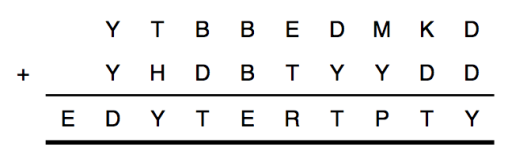
In the second problem, the equation is:
\[
YTBBEDMKD + YHDBTYYDD = EDYTERTPTY
\] In this variant, there is an “error” somewhere in the above sum. In other words, one of the letters is wrong. This seems rather difficult to model, so we will model something related (and equivalent) instead. Instead of saying that one of the letters is wrong, we’ll say that one of the column sums is wrong. Proceeding as we did in the first problem, the equations (with carry-overs) look like:
\[
\begin{array}{cccccccccc}
Q_1&Q_2&Q_3&Q_4&Q_5&Q_6&Q_7&Q_8&Q_9& \\
&Y&T&B&B&E&D&M&K&D \\
+&Y&H&D&B&T&Y&Y&D&D \\ \hline
E&D&Y&T&E&R&T&P&T&Y
\end{array}
\]Let’s introduce new binary variables $Z_1,\dots,Z_{10}$ that encode whether the corresponding column sum is incorrect or not. We want:
\begin{align}
\text{if }Z_1&=0 & &\text{then} & Q_1 &= E \\
\text{if }Z_2&=0 & &\text{then} & Q_2 + Y + Y &= 10 Q_1 + D \\
\text{if }Z_3&=0 & &\text{then} & Q_3 + T + H &= 10 Q_2 + Y \\
&\;\;\vdots & &\quad \vdots & &\;\;\vdots \\
\text{if }Z_9&=0 & &\text{then} & Q_9 + K + D &= 10 Q_8 + T \\
\text{if }Z_{10}&=0 & &\text{then} & D + D &= 10 Q_9 + Y
\end{align}Therefore, if one of the equalities does not hold, this will result in the corresponding $Z_j$ being equal to $1$. We can then add an objective function; we seek the choice of $\{Y,T,B,\dots,P\}$ and $\{Q_j\}$ and $\{Z_j\}$ such that the sum $Z_1+\dots+Z_{10}$ is minimized. We are told there is one error, so we expect to be able to achieve a sum of 1, and we’ll know where the error lies.
So how do we encode these logical “if this then that” constraints into something more manageable (i.e. something algebraic)? A popular way to do this is via the big M method. I’ll use the third constraint as an example, and let’s rearrange it so it’s equal to zero:
\begin{align}
\text{if }Z_3&=0 & &\text{then} & Q_3+T+H-10 Q_2-Y&=0
\end{align}Since $Q_2,Q_3\in\{0,1\}$ and $T,H,Y\in\{0,\dots,9\}$, by substituting in order to minimize or maximize, we obtain the following bounds:
\[
-19 \le Q_3+T+H-10 Q_2-Y \le 19
\]We can then encode the logical “if this then that” constraint as:
\[
-19Z_3 \le Q_3+T+H-10 Q_2-Y \le 19Z_3
\]Note that when $Z_3=0$, both sides of the inequality become zero, effectively turning it into an equality, which is what we wanted! Conversely, if $Z_3=1$ the left and right sides are replaced by global lower and upper bounds, so the constraint becomes a tautology. I coded this up using Julia/JuMP/Gurobi as before. The result is an integer linear program with 119 binary variables, 20 equality constraints, and 20 inequality constraints. It took about 0.3 seconds to solve on my laptop and the solution turned out to be:
\begin{align}
R&=0 & E&=1 & M&=2 & D&=3 & K&=4 \\
B&=5 & Y&=6 & H&=7 & P&=8 & T&=9
\end{align}The error occurs in the second-last column (K+D=T), which translates to (4+3=9). There are three possible ways to cause this error by changing a single letter:
If you’re just interested in the answers, here they are:
[Show Solution]
For the first problem, all four smudges must correspond to different numbers. If we relabel them as $A$, $B$, $C$, and $D$, the equation becomes:
\[
\begin{array}{cccccccc}
& E & X & M & R & E & E & K \\
+ & E & H & K & R & E & K & K \\ \hline
A & K & B & H & C & X & D & E
\end{array}
\]and the solution is given by:
\begin{align}
B &= 0 & A &= 1 & X &= 2 & K &= 3 & M &= 4 \\
C &= 5 & E &= 6 & R &= 7 & H &= 8 & D &= 9
\end{align}Or, in other words:
\[
\begin{array}{cccccccc}
& 6 & 2 & 4 & 7 & 6 & 6 & 3 \\
+ & 6 & 8 & 3 & 7 & 6 & 3 & 3 \\ \hline
1 & 3 & 0 & 8 & 5 & 2 & 9 & 6
\end{array}
\]
For the second problem, the equation is:
\[
\begin{array}{cccccccccc}
&Y&T&B&B&E&D&M&K&D \\
+&Y&H&D&B&T&Y&Y&D&D \\ \hline
E&D&Y&T&E&R&T&P&T&Y
\end{array}
\]and the solution is given by:
\begin{align}
R&=0 & E&=1 & M&=2 & D&=3 & K&=4 \\
B&=5 & Y&=6 & H&=7 & P&=8 & T&=9
\end{align}Or, in other words:
\begin{array}{cccccccccc}
&6&9&5&5&1&3&2&\color{red}{4}&3 \\
+&6&7&3&5&9&6&6&\color{red}{3}&3 \\ \hline
1&3&6&9&1&0&9&8&\color{red}{9}&6
\end{array}The error occurs on the second-last digit sum (K+D=T), which translates to (4+3=9). There are three possible ways to cause this error by changing a single letter:
I solved these problems computationally using integer programming. The first problem took 0.005 seconds and the second problem took 0.3 seconds. For comparison, exhaustively searching through all possible ways of assigning numbers to letters takes on the order of 16 seconds.
For the code, I used Julia/JuMP/Gurobi. If you are interested in seeing my code, here is my IJulia notebook.

Consider four towns arranged to form the corners of a square, where each side is 10 miles long. You own a road-building company. The state has offered you \$28 million to construct a road system linking all four towns in some way, and it costs you \$1 million to build one mile of road. Can you turn a profit if you take the job?
Extra credit: How does your business calculus change if there were five towns arranged as a pentagon? Six as a hexagon? Etc.?
Here is a longer explanation:
[Show Solution]
This is actually a famous combinatorial optimization problem with a long history. So rather than attempt to re-invent the wheel, I’ll summarize what is known about the problem and give some pointers to the relevant literature. The problem is known as the Steiner tree problem and shows up, for example, in circuit design. The problem of connecting components on a circuit board using as little wire as possible is precisely the Steiner problem!
In the graph version of the Steiner problem, you have a graph with edge weights (think of the weights as distances) and some of the nodes are labeled as “terminals”. The goal is to find a set of edges that connect all the terminals together. Not all nodes need to be part of the path. This is similar to the minimum spanning tree problem (if all nodes are terminals) or the shortest path problem (if there are only two terminals). Although these simpler variants have polynomial-time algorithms (they’re efficiently solvable), the graph version of the Steiner problem is NP-Hard. So there is likely no efficient algorithm for solving it in general. One thing we know for sure is that the optimal solution should not contain any cycles, because removing an edge from the cycle still connects the same nodes yet has a shorter path. In other words, the solution will always be a tree. This is why it’s called the “Steiner tree problem”.
If we consider the general (non-graph) version of the problem, the solution will still be a tree. A key insight is that we may need to add extra nodes to help make the path shorter. These extra nodes are called Steiner points. For example, consider the equilateral triangle case:

In this case, the version on the left has the shorter path. So we benefit from adding a Steiner point. For an arbitrary triangle, this point is called the Fermat point. The problem gets progressively more difficult as we add more terminal points. The solution for a square involves adding two Steiner points:

Some things are known about more general geometries. The following results, which I will summarize in bullet points, come from a paper from 1930 by Vojtěch Jarník. The paper is open-access so feel free to take a (free) look!
The proofs of the last two facts uses contradiction. For example, we might assume that there exists a Steiner point with three roads at angles that are not 120 degrees, and then we show that it’s possible to move that Steiner point slightly and make the total sum of the roads shorter. Therefore, we conclude that the original geometry could not have been optimal.
These facts alone aren’t enough to tell us exactly what the solutions will be, but it can help us narrow down the search! Also, it’s a quick sanity check to see whether a proposed solution can be improved in an obvious way.
Here is the solution with minimal explanation:
[Show Solution]
For an equilateral triangle, a square, and regular pentagon, the solutions have 1, 2, and 3 Steiner points, respectively. Here is what they look like:

Note that these solutions satisfy the requirements listed in the text above. Namely, each Steiner point (internal node we added) has exactly three edges emanating from it and they form angles of 120 degrees with one another. When we have a regular polygon with more than 5 sides, there are no Steiner points and the shortest road is simply the one that traverses the perimeter and leaves out one edge. For example:

This fact is proven in the following 1987 paper by Du, Hwang, and Weng.
Of course, if the polygons are not regular, all bets are off! Depending on how the points are arranged, we could have a different number of Steiner points and finding the optimal arrangement is generally very challenging.
The minimal road length for a regular polygon with sidelength $r$ is:
In the original problem statement, $n=4$ cities and $r=10$ miles. So we require 27.32 miles of road, which will cost less than \$28M to build. Therefore we do turn a profit (of about \$680k) by accepting the job.
It’s worth mentioning that this problem can also be solved with soap! Here is a neat video that explains and demonstrates it.

The famous four-color theorem states, essentially, that you can color in the regions of any map using at most four colors in such a way that no neighboring regions share a color. A computer-based proof of the theorem was offered in 1976.
Some 2,200 years earlier, the legendary Greek mathematician Archimedes described something called an Ostomachion (shown below). It’s a group of pieces, similar to tangrams, that divides a 12-by-12 square into 14 regions. The object is to rearrange the pieces into interesting shapes, such as a Tyrannosaurus rex. It’s often called the oldest known mathematical puzzle.
Your challenge today: Color in the regions of the Ostomachion square with four colors such that each color shades an equal area. (That is, each color needs to shade 36 square units.) The coloring must also satisfy the constraint that no adjacent regions are the same color.
Extra credit: How many solutions to this challenge are there?

Here are the details of how I solved the problem:
[Show Solution]
I’d like to start by pointing out that Hector Pefo also posted a nice solution to this problem. There were also diagrams of solutions posted on Twitter, such as those from @DimEarly and from @chattinthehatt. The solution I’ll describe here is similar to Hector’s, but I’ll explain how to model it as an integer linear program and solve it that way. Of course both solutions produce the same answers (because they’re both correct!) but it’s nice to see different approaches. So without further ado…
Let’s suppose there are $N$ shapes and we’d like to use $C$ colors. Define:
\[
x_{ij} = \begin{cases}1&\text{if shape }i\text{ is colored using color }j\\0&\text{otherwise}\end{cases}
\]The first constraint is that each shape must be assigned to exactly one color. We can express this algebraically as follows:
\[
\sum_{j=1}^C x_{ij} = 1\qquad\text{for }i=1,\dots,N
\]Now suppose that shape $j$ has area $a_j$. The constraint that each color has an equal share of the area means that the sum of the areas of the shapes of each color must be $A_\text{tot}/C$, where $A_\text{tot}$ is the total area of the Ostomachion. Algebraically, we can write this as:
\[
\sum_{i=1}^N a_i x_{ij} = A_\text{tot}/C\qquad\text{for }j=1,\dots,C
\]Finally, we must deal with the edge constraints. We say that $(p,q)$ is an “edge” if shape $p$ shares an edge with shape $q$. Shapes that share an edge must be different colors. We can encode this algebraically as:
\[
x_{pj} + x_{qj} \le 1\qquad\text{for all edges }(p,q)\text{ and for }j=1,\dots,C
\]And that’s it! We described the feasible set of solutions as the set of matrices $x \in \{0,1\}^{N\times C}$ that satisfy the three sets of linear constraints above. This sort of optimization model is a modified version of a Knapsack problem. More generally, it’s an Integer Linear Program (ILP). Such problems are known to be NP-hard, which roughly means that in the worst-case, there is no efficient way to solve them short of trying all possible colorings. However, modern ILP solvers are quite sophisticated and can usually solve these types of problems very efficiently.
When using an ILP model, most commercial solvers are designed to find a single solution. For this problem, we are interested in finding all solutions. One way to get around the limitation is to use Barvinok’s algorithm. One can also use variants of branch-and-cut. Yet another way, which is not as systematic but much easier to explain and implement, is to use a randomized approach.
Since all our variables are binary (0 or 1), the convex hull of the feasible set cannot contain any interior solution points. All solutions will be on the boundary. This means that any solution can be found by specifying the right objective function for the optimization. As stated, our optimization is just a feasibility problem and there is no objective specified. For this problem, we start by letting $r_{ij}$ be random numbers (we can draw them i.i.d. from a standard normal distribution, for example). Then, we simply add the objective function:
\[
\text{Minimize}\qquad \sum_{i=1}^N\sum_{j=1}^C r_{ij} x_{ij}
\]and solve the problem. If we do this repeatedly with different realizations of the $\{r_{ij}\}$, we will eventually enumerate all possible solutions of the optimization problem.
To jump straight to the solution (and pretty pictures!) see below.
[Show Solution]
I implemented the ILP described earlier using Julia and JuMP and I solved everything using the Gurobi solver. Although the randomized approach for finding all solutions works well, Gurobi has built-in functionality that allows one to directly find all solutions. In addition to doing this, I also included logic that removes duplicate solutions arising from different re-colorings of the same solution. e.g. if you take a solution and just swap red for green, I counted that as the same solution. Here are the solutions I found. I included the time it took Gurobi (on my laptop) to find all solutions for each case:
For $C=3$ colors, there are $2$ distinct solutions (took 1.6 ms to solve)

For $C=4$ colors, there are $9$ distinct solutions (took 32 ms to solve):
For $C=6$ colors, there are $33$ distinct solutions (took 700 ms to solve):

Interestingly, using fewer colors makes it easier to satisfy the equal-area constraint, but it makes it harder to satisfy the edge constraints. Ultimately, there are only solutions for the cases above ($C=3,4,6$). There are no solutions for any other values of $C$.
If you are interested in seeing my code, here is my IJulia notebook.
The following problem appeared in The Riddler and it’s about finding the right code sequence to crack open a safe.
A safe has three locks, each of which is unlocked by a card, like a hotel room door. Each lock (call them 1, 2 and 3) and can be opened using one of three key cards (A, B or C). To open the safe, each of the cards must be inserted into a lock slot and then someone must press a button labeled “Attempt To Open.”
The locks function independently. If the correct key card is inserted into a lock when the button is pressed, that lock will change state — going from locked to unlocked or unlocked to locked. If an incorrect key card is inserted in a lock when the attempt button is pressed, nothing happens — that lock will either remain locked or remain unlocked. The safe will open when all three locks are unlocked. Other than the safe opening, there is no way to know whether one, two or all three of the locks are locked.
Your job as master safecracker is to open the locked safe as efficiently as possible. What is the minimum number of button-press attempts that will guarantee that the safe opens, and what sequence of attempts should you use?
Here is my solution.
[Show Solution]
I don’t believe there is an efficient way to solve the problem (read: polynomial time), but there are efficient ways to search the space of solutions and techniques we can use to make an exhaustive search more tractable. This problem sits nicely at the boundary between what is solvable vs unsolvable via brute force. So without further ado…
First, we have to specify what it is we’re searching over. There are six possible safes, which correspond to the six permutations of (A,B,C). They are: {ABC,ACB,BAC,BCA,CAB,CBA}. Each permutation indicates which key opens which lock. For example, “BAC” is a safe where lock 1 is opened by key B, lock 2 is opened by key A, and lock 3 is opened by key C. The safe can also be in one of 8 different states, which correspond to whether each lock is currently open or closed. We can write these as binary numbers: {000,001,010,011,100,101,110,111}. For example, “010” is a safe where lock 2 is unlocked and locks 1 and 3 are locked.
Every time we make a move, we choose some assignment of the keys (A,B,C) to the locks (1,2,3). There are six possible moves we can make, which correspond to permutations of (A,B,C) as before: {ABC,ACB,BAC,BCA,CAB,CBA}. Given a hypothetical sequence of moves, we can track what happens by computing the state of the safe for each of its possible starting configurations. A simple way to track is to make a table, which I will illustrate using an example. If our safe is the “ABC” safe, and we apply the sequence of moves: ABC,CBA,BCA. The table looks like:
| ABC safe | 000 | 001 | 010 | 011 | 100 | 101 | 110 | 111 |
| ABC (111) | 111 | 110 | 101 | 100 | 011 | 010 | 001 | 000 |
| CBA (010) | 101 | 100 | 111 | 110 | 001 | 000 | 011 | 010 |
| BCA (000) | 101 | 100 | 111 | 110 | 001 | 000 | 011 | 010 |
First move (ABC): We start with a row that contains every possible state. Applying the move “ABC” will toggle all the locks, since we are working with the safe “ABC” (all keys are correct). This is equivalent to XORing the current state with the bitstring “111”. In effect, every 0 becomes 1 and vice versa, which leads us to the second row. Note that the “000” state became “111”, so the safe is opened! For the other seven initial states, the safe remains locked but is now in a different state.
Second move (CBA): this move corresponds to an XOR with “010” since only the B is in the correct position. So the third row is produced by only toggling the middle bit of the states in the second row. Here, we see that the initial state “010” leads to an open safe after the second move.
Third move (BCA): This move accomplishes nothing since none of the letters are in the correct position (XOR with “000”).
For each of the six possible safes, we can make such a table, track the evolution of each of the 8 states as the sequence of moves is applied, and keep track of which columns eventually achieve a “111” (opened safe). Each safe responds differently because the keys are matched differently to the locks. For example, if we apply the same sequence of moves to the “BAC” safe instead, we obtain:
| BAC safe | 000 | 001 | 010 | 011 | 100 | 101 | 110 | 111 |
| ABC (001) | 001 | 000 | 011 | 010 | 101 | 100 | 111 | 110 |
| CBA (000) | 001 | 000 | 011 | 010 | 101 | 100 | 111 | 110 |
| BCA (100) | 101 | 100 | 111 | 110 | 001 | 000 | 011 | 010 |
So, given a sequence of moves, we can evaluate how it affects each of the 48 possible initial states (6 safes x 8 states per safe) by computing six tables like the ones above, and then counting which columns contain “111” (the safe was opened). We can exclude the safes that start in the “111” position (safe is already open), so we only need to check 42 possible states.
The next step is to exhaustively check all possible sequences of moves, starting with shorter sequences and progressively making them longer until we find a way to make all 42 initial states eventually contain “111”. Such a search can be computationally difficult because of the “curse of dimensionality”. For example, there are $6^{12} \approx 2.18\times 10^9$ different sequences of length 12. There are several tricks we can use to reduce this burden and make the search more tractable. Here are the tricks I used:
Using the strategies above, the 2 billion possible sequences reduces to a mere 1080, a very manageable quantity. After performing the search, I found a winning sequence of length 12:
{ABC,BCA,CAB,ABC,BCA,ABC,ACB,BAC,ACB,CBA,BAC,ACB}.
The search also reveals that it’s impossible to crack all 42 states in 11 moves, so 12 is the best we can do. Finding such a winning sequence is challenging to do without a computer. Two observations: