This Riddler is about microorganisms multiplying. Will they thrive or will the species go extinct?
At the beginning of time, there is a single microorganism. Each day, every member of this species either splits into two copies of itself or dies. If the probability of multiplication is p, what are the chances that this species goes extinct?
Here is my solution:
[Show Solution]
Here is a short and sweet solution to the problem. Let’s call $q$ the probability that the species eventually goes extinct. If a microorganism fails to multiply (probability $1-p$), then it goes extinct immediately. If it multiplies, we now have two microorganisms, each with probability $q$ of eventually going extinct. The probability that they both eventually go extinct is $q^2$ because they behave independently. Therefore, we can write the recursion:
\[
q = p\, q^2+(1-p)
\]This equation has two possible solutions: $q \in \{1, \tfrac{1}{p}-1\}$. Since probabilities cannot exceed $1$, the second solution only makes sense in the case where $p \ge \tfrac{1}{2}$. Therefore, the solution is:
\[
q = \begin{cases}
1 &\text{if }p < \tfrac{1}{2} \\
\tfrac{1}{p}-1 &\text{if }p \ge \tfrac{1}{2}
\end{cases}
\]Here is a plot showing what the probability of extinction looks like as a function of $p$, the probability of multiplication:
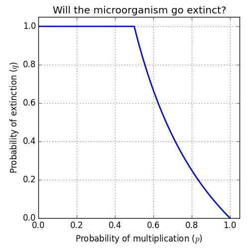
This is an interesting result because of the phase transition that occurs at $p=\tfrac{1}{2}$. If the probability of multiplication is less than one half, the species will always eventually go extinct. When the probability of multiplication is greater than one half, there is a nonzero chance that the population will grow enough that the species becomes “too big to fail”.
Here is a more technical (and more correct!) solution adapted from a comment by Bojan.
[Show Solution]
The previous approach obtains the correct answer, but the issue of which solution to the quadratic equation to pick still remains. This alternative approach obtains the correct answer using a generating function approach. Define the probability distribution:
\[
P_n(i) := (\text{probability there are }i\text{ microorganisms on day }n)
\]Now define the sequence of polynomials:
\[
Q_n(x) := \sum_{i=0}^\infty P_n(i)\, x^i
\]Then $Q_1(x) = x$, since there is one organism on day one. We can derive a recursive relation for the multiplication/exctinction process by thinking carefully about how the population can change from one day to the next. It’s not difficult to see that after the first timestep, the population must always be even. If the population is $2i$ at time $n+1$ and the population was $j$ at time $n$, then $j \ge i$. The probability that we transition from $j$ to $2i$ requires that exactly $i$ microorganisms multiply and the rest die. This can happen in ${j\choose i}$ ways, each with probability $p^i(1-p)^{j-i}$ (it’s a binomial distribution). Therefore, we have the recursion:
\[
P_{n+1}(2i) = \sum_{j=i}^\infty {j\choose i} p^i (1-p)^{j-i} P_n(j)
\]We can now use this fact to find a recursion for our generating function $Q_n.$ Again, we’ll make use of the fact that when $n>1$, there can only be an even number of microorganisms:
\begin{align}
Q_{n+1}(x)
&= \sum_{i=0}^\infty P_{n+1}(i)\, x^i\\
&= \sum_{i=0}^\infty P_{n+1}(2i)\, x^{2i}\\
&= \sum_{i=0}^\infty \sum_{j=i}^\infty {j\choose i} p^i (1-p)^{j-i} P_n(j)\, x^{2i} \\
&= \sum_{j=0}^\infty \sum_{i=0}^j {j\choose i} p^i (1-p)^{j-i} P_n(j)\, x^{2i} \\
&= \sum_{j=0}^\infty P_n(j) \sum_{i=0}^j {j\choose i} (px^2)^i (1-p)^{j-i} \\
&= \sum_{j=0}^\infty P_n(j) \left(px^2+(1-p)\right)^j \\
&= Q_n(px^2+(1-p))
\end{align}A couple notes: in the fourth step, we interchanged the order of summation for $i$ and $j$ and in the sixth step we used the binomial theorem. Summarizing, we conclude that
\[
Q_{n+1}(x) = Q_n(px^2+(1-p))
\]The probability of extinction after $n$ timesteps is $P_n(0)$ (the probability that the population is zero). We’re interested in the limit of $P_n(0)$ as $n$ goes to infinity. This is equivalent to the constant term in our sequence of polynomials, so we are interested in finding: $\lim_{n\to\infty} Q_n(0)$. Let’s take a look at the first few terms:
\begin{align}
Q_1(x) &= x\\
Q_2(x) &= px^2 + (1-p)\\
Q_3(x) &= p\left(px^2 + (1-p)\right)^2 + (1-p)\\
Q_4(x) &= p\left(p\left(\left(px^2 + (1-p)\right)^2 + (1-p)\right)^2 + (1-p)\right)^2 + (1-p)\\
\dots
\end{align}Evaluating at zero, we get:
\begin{align}
Q_1(0) &= 0\\
Q_2(0) &= 1-p\\
Q_3(0) &= p(1-p)^2 + (1-p)\\
Q_4(0) &= p\left( p(1-p)^2 + (1-p)\right)^2 + (1-p)\\
\dots
\end{align}The pattern is clear (we could also prove it using induction). If we define $q_n := Q_n(0)$, the recursion satisfied is:
\[
q_{n+1} = p\, q_n^2 + (1-p)\qquad\text{with: }q_1 = 0
\]Any limit $q_n \to q$ of this recursive sequence must satisfy the fixed point equation $q = p\,q^2+(1-p)$. This is precisely what we found in our first solution to the problem! So what’s the big deal? Why did we go through all this trouble to arrive at the same answer?? This recursion actually tells us something more that just the limiting case. It tells us how we approach the limiting case. In other words, it gives us the dynamics.
Let’s take a closer look at these dynamics in the neighborhood of the two fixed points $q=1$ and $q=\tfrac{1}{p}-1$. If we let $\delta_n := q_n-1$, we can rewrite the recursion as:
\[
\delta_{n+1} = 2p\, \delta_n + p\, \delta_n^2
\]Of course, if $\delta_n=0$ (i.e. $q_n=1$), then it will remain at $1$ forever. But what if we are merely close to this fixed point? Then $\delta_n \approx 0$ and we have $\delta_{n+1} \approx 2p\,\delta_n$. Notice that when $p > \tfrac{1}{2}$ If $\delta_n$ is close to zero, it will never get closer because $2p > 1$. These dynamics are unstable.
Now take a look at the other fixed point. If we let $\epsilon_n := q_n-\tfrac{1}{p}+1$, then we can rewrite the recursion as:
\[
\epsilon_{n+1} = 2(1-p)\epsilon_n + p\,\epsilon_n^2
\]If we are close to this fixed point, then $\epsilon_n \approx 0$ and we have $\epsilon_{n+1} \approx 2(1-p)\epsilon_n$. This time, when $p > \tfrac{1}{2}$, we have $2(1-p) < 1$. In other words, if we are close, we continue to get closer! These dynamics are stable.
This stability argument explains why we converge to $\tfrac{1}{p}-1$ rather than $1$ in the case where $p>\tfrac{1}{2}$. If we consider the other case, where $p<\tfrac{1}{2}$, the stability flips. The first fixed point becomes stable and the second one becomes unstable. This transition in stability of the dynamics explains the abrupt transition in the plot at the point $p=\tfrac{1}{2}$.
Laurent,
Very elegantly done! There is one small error in your explanation: it’s because a probability must be less than or equal to one (not that it must be non-negative), that the second solution of the quadratic equation only makes sense if p is greater than or equal to 1/2.
Thanks! fixed it.
Hey Riddlers, I think there may be more than a quibble here! True, (1/p – 1) is a probability only for p greater than or equal to 1/2, but of course 1 is also always a probability. How do we know that the switch from probability 1 to (1/p – 1) happens at a p = 1/2 rather than 3/4 or even right at 1?
I’m not sure that the technique Laurent uses (which I admit I also until now thought was fine) can by itself rule out the probability of extinction being 1 for any p. The quadratic is satisfied by 1 for any value of p; and so are the polynomial equations you get with similarly-motivated expressions for the probabilities of populations of size 2, 4, 6, etc., going extinct. It’s not hard to see why, once you think about it. These equations say that the probability of extinction, say for a population of size n, is a weighted mixture of 1 for sudden extinction (weighted by probability (1-p)^n) and the various probabilities of extinction for the different non-zero sizes the population might next reach (weighted by the probabilities of reaching those sizes). If these extinction probabilities are all 1, we have a weighted mixture of 1s with weights that sum to 1, which sums to 1.
So it looks like we need another insight?
Good point. This did occur to me at the time and I never quite figured out how to reconcile the multiple solutions in the case $p > 1/2$. I did simulate the problem numerically and found that the solution undergoes a transition at $p=1/2$ as I indicated in my write-up… but I don’t have any better insight at the moment. Let me know if you figure anything out!
Here’s an argument that the transition occurs at p=1/2: Suppose we have N organisms. Each has probability p to become 2, and probability 1-p to become zero; hence the expected number of organisms the next day is 2pN. So if we start with one organism on day zero, the expected number on day k is (2p)^k. If extinction happens with probability 1, the expected number must go to zero at large k. This happens only for p<1/2.
Nice! That makes the curve much easier to understand. While the expected population for large k goes to infinity for all p>1/2, that’s compatible with nonzero probability (even with near certainty) of extinction. That’s a lot like the St. Petersburg “paradox,” where you get 2^n dollars for throwing your first tails at the nth coin toss (the expectation is infinite even though you’re nearly certain not to get more than 1000 dollars).
That’s a good thought, MarkS, but it’s not quite correct here. You could have a situation where extinction happens with probability 1, but the expected population size goes to infinity. (eg. If all organisms divide in two at every time step but there is a probability p of extinction at each time step. If p 0, extinction occurs almost surely.) Without getting into the measure theoretic details, you need some additional conditions to say that the expected population size must go to 0 if extinction occurs with probability 1.
In this case, you can define q_n to be probability the population is extinct at time n. Then you have the same recursive equation: q_n = (1-p) + p q_{n-1}^2. Since q_0 = 0, you can show by induction that q_n <= 1/p-1 for all n, so q = lim q_n <= 1/p-1.
Well done, Laurent! I was thigh-deep in Markov chains, but simulations bolster your formula.
Your blog is alway very illuminating. I’m still confused about the equation you used to solve q, why stop at the first generation and not include the second generation and so on?
Hi Gabriel,
In my solution, $q$ is the probability that the species eventually goes extinct. Therefore, $q$ already takes into account all future generations. For a particular microorganism to go extinct, all of its descendants must eventually fail to reproduce. The key insight is that when a microorganism does reproduce, the two new microorganisms are like separate populations that are starting from scratch, and so each has probability $q$ to eventually go extinct.
Hello,
an alternative way to determine the “correct” solution to the quadratic equation for $p>1/2$ is to explicitly calculate the population distribution on any given day. Say,
\[
Q_n(x) = \sum_{i=0}^\infty x^i \cdot (\text{probability there are }i\text{ microorganisms on day }n).
\]Then $Q_1(x) = x$, since there is one organism on day one. And, the recursive relation governing the multiplication/extinction process is
\[
Q_{n+1}(x) = Q_n(px^2+(1-p)).\qquad\qquad(1)
\]The probability of extinction is $\lim_{n\to\infty} Q_n(0)$ and can be easily shown to be what you have calculated (using $Q_1(x)=x$ and $(1)$).
This is wonderful, thank you! I reformatted your comment using LaTeX (you can do so yourself in the future by typing comments in LaTeX directly!). I also added an extra solution in my blog post inspired by your generating function approach. There is probably a more direct way of deriving the dynamics than what I did, but it was still a fun exercise to work through. This way of solving the problem clearly shows why we transition from one solution to the other; it’s all about stable vs unstable equilibria.
I have a few thoughts here.
First, this problem is akin to the Cliff Hanger (problem 35) in Mosteller’s Fifty Challenging Problems in Probability. Even the graph on page 53 of the book is identical to the one on LL’s blog here. I love this little book, so I didn’t spend that much time directly on this problem. The caveat is, what I am about to say may make more sense, directly speaking, in context of the cliff hanger problem.
Second respect to some of the comments, like which root of the quadratic equation to choose, I have two thoughts.
A) Mosteller says in his book that for the curve depicted in LL’s blog to avoid jumps, it must adopt $(1-p)/p$ for $p\gt 1/2$. That is the selection of which root to choose reduces to showing that your probability function itself does not have jumps.
B) As much as I like Mosteller, I’d suggest at least considering a simpler approach.
My take is to consider instead using a ‘loose’ upper bound. My only requirement is to avoid the degenerate cases of $p = 1$ and $p = 0$. (And we can know the results from those deterministic cases without any further analysis simply by eyeballing things.)
What’s the probability of failure in the first move? $1-p$. We can of course upper bound this with… 1-p. What’s the probability of instead failing as soon as possible after that (i.e. go up once, then down twice). Most would say we can use $p(1-p)^2$. I would say let’s upper bound this with $(1-p)^2$. Howabout the probability of failing not at the first possible time or the second feasible time but instead on the third feasible time? I would say let’s take it easy and upper bound this by $(1-p)^3$. And I would say that we can upper bound the next failure by $(1-p)^4$… and we can upper bound the kth failure by $(1-p)^k$. Thus, in the limit, if we want the upper bound on the total probability of failure, it is given by the geometric series of
$y = (1-p) + (1-p)^2 + (1-p)^3 + (1-p)^4 + (1-p)^5 + …. $
Again for non-degenerate probabilities, we know we’re in the radius of convergence of the geometric series. Accordingly, we can say that the *upper bound* on the probability of failure is
$y = \frac{1-p}{p}$
It may be quite instructive to plot this on a graph, but you can clearly see that this upper bound is greater than $1$ when $p\lt 0.5$. This upper bound means we can safely ignore the root value of 1 when $p > 0.5$. (The fact that this ‘loose’ upper bound is equal to the lower bound when $p \geq 0.5$ is outside the scope.)
hmmm… not sure what happened here. It seems that greater than (but not $\geq$) or less than signs (but not $\leq$) in LaTeX are causing issues to make text disappear… ?
For clarity, my last paragraph should read:
– – – –
It may be quite instructive to plot this on a graph, but you can clearly see that this upper bound is $\leq 1$ when $p \geq 0.5$, with equality only at p = 0.5. This upper bound means we can safely ignore the root value of 1 when p >0.5. (The fact that this ‘loose’ upper bound is equal to the lower bound when p≥0.5 is outside the scope.)
WordPress interprets the less-than and greater-than symbols as html syntax, which is why it’s causing problems. If you want to use that symbol in $\LaTeX$ math mode, simply use \lt and \gt for $\lt$ and $\gt$ respectively. I updated your original post.
Thank you for your comment! I found Mosteller’s Cliffhanger problem online; basically it’s a random walk problem where you walk “away” from the cliff with probability $p$ and “toward” the cliff with probability $1-p$. The question is to find the probability that you’ll walk off the cliff eventually. In the Cliffhanger problem, you only take one step at a time, but this is equivalent to the microorganism problem if you just assume that the microorganisms choose their individual fates sequentially! Very neat.
Yea…. my bounding with geometric series idea seems to need some work though. As is, I don’t like it anymore!
It’s been a long day.
Thanks for the note on LaTeX. I’m so used to typing LaTeX in Jupyter notebooks, I completely forgot about the possibility of symbolic collision with HTML!
– – – – –
Here is another approach to the cliffhanger problem. It involves a bit more machinery, but I think this sketch nicely decomposes what is going on in this process. Sorry for the length, but I saw a ballot problem hiding in here so I had to do it!
—— – –
As always, I am not interested in degenerate probabilities, so I again assert that $p \neq 0$ and $p \neq 1$. We can simply eyeball those cases. I will also suggest that we can think of this game (the ‘cliffhanger game’) as being a finite iterative one having n + 2 states: where the different states are: $\{-1, 0, 1, 2, …, n-1, n\}$, and we play it for n iterations. (E.g. if n = 1, we have states {-1, 0, 1,}, we start at state 0, and play for 1 iteration.) In all cases we start at state zero. If we ever visit state $-1$ during an iteration, the game is a failure.
The final game that is posed then asked for what happens $\lim_{n \to \infty}$. Note that the official problem merely suggests starting with countably infinite number of states, but I generally find that starting with a finite number and considering the limitting process can help clarify your thinking. (As I recall Jaynes would *insist* that we try to do this.) If people are worried about pathologies, they can consider approaching this limit from different orientations to confirm.
For my setup, there are some underlying ideas of linear independence and requiring the possibility of traversing the graph for n iterations without having a cycle that motivate this approach for this problem. (That is, for a finite graph, the state n will in effect be viewed as an absorbing state. But since we always start at state 0 and only allow n iterations, we can never hit state n on anything except the final iteration — so transition probabilities from state n are not relevant, by design. If we were for some reason starting on state 1 instead, I would insist that the there be n + 3 states with n iterations… in any case the translation needed to accomodate a different starting point, or different failure point is quite simple.)
The interesting thing about this approach is it clarifies the mechanics of what is going on in the process — in effect it acts like a decomposition.
So first, consider our expected position after n iterations. Note that expected position change per iteration is $2p – 1$, and we have $n$ i.i.d. processes going on here. It’s not really needed, but I’ll mention that the variance of position change per iteration is given by $4(p – p^2)$.
The expected position / drift, at $n$ iterations is given by $\mu = n\big(1*p + -1*(1-p)\big) = n (2p – 1)$. Similarly we can say that the expected position is given by $\mu = ExpectedUpSteps – ExpectedDownSteps$, where $np = ExpectedUpSteps$ and $n(1-p) = ExpectedDownSteps$. There is probably a touch more care needed at this stage than I’m willing to put in this post, to highlight that I will also look at $\bar X$ which is the average result per iteration (aka $\frac{\mu}{n}$). For the most part, using $\bar X$ is preferable to $\mu$ because it converges — but I’ll toggle the representation as expediency indicates I should. I’m inclined to call $\mu$ drift and $\bar X$ average drift.
From here we can use the strong law of large numbers or the weak law of large numbers or convergence in mean squared error — it doesn’t really matter– and notice that as n grows large, there is a vanishly small chance of having an average move size other than $\bar X$.
Thus we can decompose this problem into $(a)$ looking at the average drift of the process and $(b)$ looking at the chances of hitting the state $\{-1\}$ during an intermediate step. Loosely speaking $(a)$ refers to long-run behavior, while $(b)$ is oriented to problems that occur in the short-run. Our interest is solely what happens when $n$ grows large (and not, for instance, in the rate of this convergence).
From this we can immediately see from our formula $\bar X = (2p – 1) \lt 0$, if $p \lt 0.5$. From $(a)$ alone we can see that the probability of failure goes to 1 as $n$ grows large, for any $p \lt 0.5$. Put most simply, and accurately, if our average results converge on $\bar X$, and $\bar X \lt 0$ then that implies we must have more -1s than +1 in our sample path at some point. This is means a failure must have occurred. The intricacies of $(b)$ simply are not relevant here. (The underlying idea I want to emphasize here is that the long-run behavior given by component $(a)$– the average drift– dominates and causes failure for $p \lt 0.5$.)
– – – –
Now consider the case where $p \geq 0.5$. The $p = 0.5$ case indicates zero drift, and the $p \gt 0.5$ case indicates positive drift. In these cases, $\mu$ alone won’t cause failure as n grows large, so we need to consider $(b)$. What’s interesting is that $(b)$ is a ballot problem! Put differently, we can use the reflection principle here. A sketch follows:
where you have $ r = StepsDown$, $k = StepsUp$ and $s = DownStepsTillFailureGivenStart$. Note for our problem $s := 1$ but I’ll consider a more general formula.
The idea is that for any given full iteration of the model, total moves $ = n = r + k$. There are $\binom{n}{k} = \binom{r + k}{k}$ ways to choose any particular sequence of moves. So given that you are in some particular position (specifically your expected position), the probability of failure is given by the number of moves that cause failure and get you to your position divided by total number of possible ways to get to your position.
The formula for this is: $\binom{r + k}{r – s} \binom{r + k}{k} ^{-1} = \frac{\binom{r + k}{r – s}}{\binom{r + k}{k}}$
Since in our case $s$ is always equal to 1 (i.e. we always start at state zero, and a failure is one downward step away), we can rewrite this as:
$\binom{r + k}{r – 1} \binom{r + k}{k} ^{-1} = \frac{k!r!}{(r – 1)! (k+1)!} = \frac{r}{k+1}$
so the formula for probability of failure in the case of non-negative drift is given by: $\frac{r}{k+1}$
It’s worth highlighting that, for ballot problems the size of r and k matter! Inserting something akin to $\bar X$ instead of $\mu$ does not line up with the physical meaning of the ballot problem. It truly wants the total number of yays vs nays that exist (for any given n).
Now it’s a matter of considering that as n grows large, the average value we see with probability one is $\bar X$, and we can decompose this into the average of up steps and average downs steps. To align with the physical meaning of the ballot problem, we will scale these values up appropriately (i.e. by $n$). Thus we make the following two assignments:
$r:= ExpectedDownsteps = n(1-p) $
$k:= ExpectedUpsteps = np$
$\frac{(r)}{(k)+1} = \frac{\big(n(1-p)\big)}{\big(np \big)+1}$.
Again recalling that I’ve banished degenerate probabilities from this post, distilling the answer just requires a simple limit:
$Probability_{Failure} \big| p \geq 0.5 = \lim_{n \to \infty} \frac{n(1-p)}{np+1} = \lim_{n \to \infty}\frac{(1-p)}{p + \frac{1}{n}} = \lim_{n \to \infty}\frac{(1-p)}{p + O \big(\frac{1}{n}\big)} = \frac{1-p}{p}$
From here it’s just a small bit of work to consider the general case of $s$ moves until failure from a given start. For any natural number $s \geq 1$, this general failure probability equals
$Probability_{Failure} \big| p \geq 0.5 = \lim_{n \to \infty}\frac{n^s(1-p)^s + O\big(n^{s-1}\big)}{n^s p^s + O\big(n^{s-1}\big) } = \lim_{n \to \infty}\frac{(1-p)^s + O \big(\frac{1}{n}\big)}{p^s + O \big(\frac{1}{n}\big)} = \Big(\frac{1-p}{p}\Big)^s$
– – – –
Hopefully this viewpoint is complementary to the original solution by LL on this matter, and gives some additional insight as to why there is a breakpoint in probability of failure at $p = 0.5$. I suppose that there may be a bit of overlap with the generating function approach, though try as I might, generating functions don’t really speak to me. I also rather like ballot problems 😉
Nice!
Interestingly, I didn’t find a direct way to prove which is the right solution to the quadratic equation for Mosteller’s Cliffhanger problem.
Using this analogy, and the proof to the organism problem we get a full solution to the Cliffhanger as well.
By the way: here is a more technically careful way to deal with the ballot problem at the end of my writeup when I said:
$\binom{r + k}{r – 1} \binom{r + k}{k} ^{-1} = \frac{k!r!}{(r – 1)! (k+1)!} = \frac{r}{k+1}$
or in general
$\binom{r + k}{r – s} \binom{r + k}{k} ^{-1} = \frac{k!r!}{(r – s)! (k+s)!} = \frac{r^s + O(r^{s-1})}{k^s + O(k^{s-1})}$
From here observe that we are doing this ballot problem for a sequence of modified bernouli trials ($\{-1,1\}$ vs $\{0,1\}$ is just a small boolean modification). But what the ballot formula tells us, is for any sequence of iid bernouli-ish trials, with a stationary lower ‘knockout’ barrier, as $n$ grows large, all that matters is the ratio between $r$ and $s$. That is
$\lim_{n \to \infty} \frac{r^s + O(r^{s-1})}{k^s + O(k^{s-1})} =\big( \frac{r}{k}\big)^s $
To justify this, observe first that $n = k + r$, where $k \geq 0$, $r \geq 0$. Thus for $n$ to grow large, at least one of $k$ and $r$ must grow large. However, if one of $k$ or $r$ grows large, but not the other, then a contradiction (or really a zero probability event) is raised. (It is perhaps worth mentioning that in the case of $r \gt k$, we don’t need the formula for the ballot problem — quite simply if $r \gt k$ then you have a negative number and any negative number indicates failure. If this were a binomial option pricing model for barrier options this technical nit would be dealt with via an if statement. In any case, if as n grows large, and $p \gt 0.5$, then the probability of $\frac{r}{k} \geq 1$ goes to zero.)
Specifically, we know $\lim_{n \to \infty} Pr\big\{ \big| SampleMean – \bar X \big| \gt \epsilon \big\} = 0$ for every $\epsilon \gt 0$, by Weak Law of Large Numbers. Hence the only non-zero probability outcome event is when $k$ and and $r$ grow aribtrarily large as $n$ grows arbitrarily large (and do so in proportion to their respective probabilities).
So the idea that the ballot problem tells us, is that in the limit, the relative proportion between $r$ and $k$ is what matters. Thankfully we know this is baked into $\bar X$. This is particularly easy to see since we have binary payoffs. Again, if our mixture of ups vs downs was anything other than p and 1-p, our sample mean in $\lim_{n \to \infty}$ would not equal $\bar X$. Hence we can make a substitution into $\frac{r}{k} = \frac{1-p}{p}$, and consider in the general case that the answer is given by $\Big( \frac{1-p}{p}\Big) ^s$, for any natural number $s \geq 1$.
Hi,
I believe I found a similar, but slightly simpler solution:
(I will not use LaTeX, feel free to edit my comment)
First, define q_n as the probability of extinction at time point n.
So q_1 = 0, q_2 = 1-p.
Using basic probability we have (1): q_(n+1) = (1 – p) + p * q_n ^ 2
In words: the probability of extinction at point n+1 equals to the sum of two probabilities:
A. The first cell dies immediately: 1-p.
B. The first cell survives and both offsprings’ subcultures are extinct at their point n: p * q_n * q_n.
Now we find the limit.
First, the limit exists because {q_n} is increasing and bounded (e.g. by 1).
The limit must satisfy x = (1 – p) + p * x^2, therefore it is either 1 or Q = 1/p – 1.
Now to prove that when p > 0.5 the limit can only be Q = 1/p – 1 we note that, by induction, {q_n} is bounded by Q.
That’s it.